RDP 2021-05: Central Bank Communication: One Size Does Not Fit All Appendix D: Model Validation Results
May 2021
- Download the Paper 2,051KB
D.1 Confusion matrix
We apply our fine-tuned RF models to the validation dataset and the prediction results are shown in the confusion matrices in Tables D1 and D2. Using the confusion matrix, we can calculate a number of performance metrics, such as:
- Accuracy: the proportion of the total number of predictions that were correct. That is the sum of true positive (TP) and true negative (TN) divided by the total observations (TP+TN+FP+FN). In Table D1 (reasoning panel), the accuracy is calculated as: (33 + 23) / (33 + 13 + 4 + 23) = 76.71%.
- Sensitivity: the proportion of postives that are correctly predicted. In Table D1, the sensitivity is calculated as (33) / (33 + 4) = 89.19%.
- Specificity: the proportion of negatives that were correctly predicted. In Table D1, the sensitivity is calculated as (23) / (13 + 23) = 63.89%.
Kappa is another metric that can be calculated from the confusion matrix using the formula:
where:
Accuracy is a fairly commonly used measure and it varies from 76.7 per cent for the economist content model to 65.2 per cent for the non-economist clarity model; 70 per cent is a threshold usually considered to indicate ‘fair’ performance.[27] A final validation measure included in these tables, but which can not be calculated directly from the confusion matrix because it focuses on the strength of the prediction, is LogLoss[28] – lower numbers are better for this metric. Overall, our results on this metric are relatively poor, reflecting the fact that our model does not make strong predictions about paragraph quality.
| Reasoning | Readability | |||||||
|---|---|---|---|---|---|---|---|---|
| Confusion matrix | Performance measures |
Confusion matrix | Performance measures |
|||||
| Reference | Reference | |||||||
| Prediction | High | Low | Accuracy = 76.71% | Prediction | High | Low | Accuracy = 72.37% | |
| High | 33 | 13 | 95% CI: (65%, 86%) | High | 28 | 11 | 95% CI: (61%, 82%) | |
| Low | 4 | 23 | Sensitivity = 89.19% | Low | 10 | 27 | Sensitivity = 73.68% | |
| Specificity = 63.89% | Specificity = 71.05% | |||||||
| Kappa = 0.53 | Kappa = 0.45 | |||||||
| LogLoss = 0.75 | LogLoss = 0.80 | |||||||
| Reasoning | Readability | |||||||
|---|---|---|---|---|---|---|---|---|
| Confusion matrix | Performance measures |
Confusion matrix | Performance measures |
|||||
| Reference | Reference | |||||||
| Prediction | High | Low | Accuracy = 69.91% | Prediction | High | Low | Accuracy = 65.22% | |
| High | 41 | 18 | 95% CI: (61%, 78%) | High | 48 | 27 | 95% CI: (56%, 74%) | |
| Low | 16 | 38 | Sensitivity = 71.93% | Low | 13 | 27 | Sensitivity = 78.69% | |
| Specificity = 67.86% | Specificity = 50% | |||||||
| Kappa = 0.40 | Kappa = 0.29 | |||||||
| LogLoss = 0.82 | LogLoss = 0.61 | |||||||
D.2 ROC-AUC
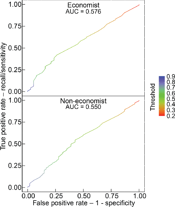
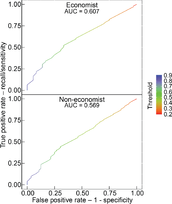
ROC is a probability curve that plots the false positive rate (FPR) on the x-axis and the true positive rate (TPR) on the y-axis for different probability cut-off thresholds. The area under the curve (AUC) is a measure of separability that is calculated as the area under the curve. The higher the AUC, the better the model is at definitively distinguishing between paragraphs with high quality and low quality. For a random classifier, such as a coin flip, there is a 50 per cent chance to get the classification right, so the FPR and TPR are the same no matter which threshold you choose. In this case the ROC curve is the 45-degree diagonal line and the area under the curve (AUC) equals 0.5. Thus, we would like to achieve an AUC of above 0.5. Our results, as shown in Figures D1 and D2, beat this benchmark but not substantially.
The fundamental problem we face in using the AUC metric is that the underlying quality of paragraphs is not cleanly separated into high and low, but has a large mass of inherently ambiguous paragraphs. What AUC requires is that a paragraph that is of ‘51% quality’ is always perfectly classified as high while a paragraph of ‘49% quality’ is always classified as low, regardless of the cut-off threshold you use with your algorithm. For example, our algorithm may report that there is a 51 per cent chance that a given (truly 51% quality) paragraph is of high quality. We use a threshold of 50 per cent and this paragraph would be correctly classified as high with that cut-off. But, the AUC also asks what if you used a cut-off of 55 per cent, of 60 per cent and so on – it is calculated for all possible cut-offs between 0 per cent and 100 per cent. The AUC will find that if you use any threshold above 51 per cent it will misclassify the paragraph and this leads to a low AUC measure for this problem. Thus, while AUC is a standard metric, it is not a good metric for our particular problem given the underlying data is not a binary variable but closer to a continuous variable. For the same reason, the LogLoss values – an alternative metric – are a bit high, ranging from 0.6 to 0.8. Notwithstanding this, we anticipate that further refinements of the algorithm should be possible that improve its performance on these and other metrics.
It is also important to note that our models report a relatively high accuracy when we set the threshold at 0.5. That is, while our model does not do a good job at neatly separating high- and low-quality paragraphs at every threshold, it does a reasonable job of identifying paragraphs that are more likely than not to be high or low quality. In this respect it is quite ‘human-like’. This suggests that the results for any given paragraph should not be given a large weight but, with a large enough sample, the results will still be useful.

Note: The ROC curve as a matrix, where the first column contains the false positive rate, the second contains recall (sensitivity) and the third contains the corresponding threshold on the scores (shown as colour in each panel)
Source: Authors' calculations using survey results

Note: The ROC curve as a matrix, where the first column contains the false positive rate, the second contains recall (sensitivity) and the third contains the corresponding threshold on the scores (shown as colour in each panel)
Source: Authors' calculations using survey results
Footnotes
We also applied the other algorithms discussed in Section 6.1 to our validation dataset for the economist content model and their accuracy was worse than our final model (the fine-tuned RF model). For more details, please refer to the online supplementary information. [27]
LogLoss is another metric that is widely used for assessing prediction performance of ML models. It is calculated as: where yi is the label and p(yi) is the predication probability. LogLoss penalises false classification, especially heavily on those that are confidently wrong. It ranges from zero to infinity. [28]