RDP 2018-01: A Density-based Estimator of Core/Periphery Network Structures: Analysing the Australian Interbank Market 6. Numerical Analysis of Core/Periphery Estimators

Sections 4.4 and 5 assess inaccuracy when the network consists of a continuum of representative true-core banks and a continuum of representative true-periphery banks. Moreover, these sections only evaluate the CvP and DB estimators. To evaluate the performance of all four of the previously discussed estimators, and to assess inaccuracy when networks have a finite number of non-representative banks, we conduct a numerical analysis.

To perform our numerical analysis, we construct 10,000 random draws from a distribution of ‘feasible’ networks. From Section 3, the average number of active banks in our quarterly data is around 40, and the average network density is 0.25. So we restrict feasibility to be networks with N = 40 banks and a density of d = 0.25. We then evaluate the performance of the estimators for various possible true-core sizes (i.e. we construct 10,000 draws for each true-core size).

We incorporate noise by allowing the densities of links within the true-core and true-periphery blocks to randomly deviate from their ideal densities. However, we do not want these densities to deviate so far from an ideal CP structure that the CP model becomes inappropriate; so we impose d_C > d_O > d_P (consistent with Section 4.4). With quarterly networks aggregated from high-frequency data, noise is more likely to come in the form of additional links rather than missing links; so we restrict the noise in the true-core block to be less than the noise in the true-periphery block (i.e. 1 − d_C < d_P).^[22] Once the densities of each block are determined, links are assigned based on an Erdős-Rényi model.^[23] Appendix D details the process for constructing simulation draws.

With 40 banks, the number of potential CP splits is 2⁴⁰ = 1 099 511 627 776 (each of the 40 banks is either a core bank or a periphery bank). So it is not feasible to search through all possible partitions to find the global optimum of each estimator. Instead, for each estimator and for each draw from the distribution of feasible networks, we construct 20 random starting points and run a ‘greedy algorithm’ to find the local optimum associated with each starting point.^[24] As a result, each estimator's performance will depend on both its theoretical properties and on how easy it is for the greedy algorithm to find a global optimum.

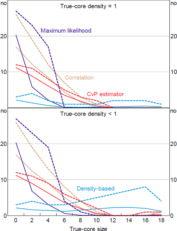
Figure 6 shows the number of banks incorrectly classified by each estimator.^[25] The top panel shows the results when there are no missing links in the true-core block (d_C = 1), the bottom panel shows the results when missing links are allowed within the true-core block (d_C < 1). Even if an estimator accurately determines the size of the core, if it puts the wrong banks in the core then it will register a positive error in this figure.

When the true size of the core is small, the DB estimator is the most accurate; especially given that the noise is added in a way that advantages the maximum likelihood estimator. The relative accuracy of the DB estimator at small core sizes is even higher when looking at the 95th percentiles. At larger core sizes, the DB estimator is slightly less accurate than the other estimators, with the accuracy differential becoming more acute when noise is added to the true core. So no estimator is unambiguously the best, which is problematic given that the true-core size and the volume of noise in real-world networks are unknown.

That said, the accuracy differential when the true core is large is never as high as the differential when the true core is small. And the areas under the DB estimator's error curves in Figure 6 are much lower than the areas under the other estimators' error curves (for both the averages and 95th percentiles).^[26] Therefore, the DB estimator is the superior estimator when no prior information about the true size of the core is available.

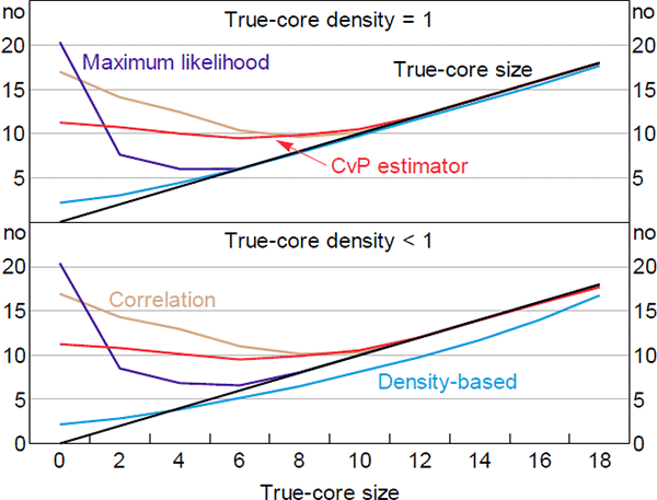
Figure 7 shows how the estimated core sizes relate to the true-core sizes (on average). Adding noise to the true-core block (bottom panel) magnifies the average underestimate exhibited by the DB estimator at larger true-core sizes. An underestimate occurs when some true-core banks have a sufficiently small number of links (relative to the other true-core banks) that moving them into the periphery reduces the core error-density by more than it increases the periphery error-density. This is more likely to occur when there are fewer links within the true core (i.e. when the amount of noise in the true-core block increases).

Importantly, the bias exhibited by the DB estimator is relatively stable across true-core sizes. So our DB estimator is likely the best method for evaluating changes in the size of the core over time.

With respect to the CvP estimator, these numerical results are consistent with the theoretical results of Section 4.4. First, the CvP estimator is theoretically inaccurate when the density of the network is high relative to the true size of the core; in the simulations the network density is fixed, so this occurs at small true-core sizes. Second, the inaccuracy is theoretically worse the further the density of the network deviates from the true proportion of banks in the core; in the simulations this translates into the inaccuracy worsening as the true-core size decreases, which is what we observe.

Given the superior performance of our estimator in both these numerical simulations and the earlier theoretical analysis, we use the DB estimator for our analysis of the Australian overnight interbank market.

Footnotes

For a pair of banks, a link occurs if there is at least one loan during a quarter, a missing link only occurs if there is never a loan during the quarter. [22]

This advantages the maximum likelihood estimator that has this as a parametric assumption. Using another network model to introduce noise is akin to imposing a probability distribution on the residual in a linear regression model. [23]

From a given starting point, a greedy algorithm searches through all possible single changes (i.e. changing a single bank from core to periphery, or vice versa) and determines the change that optimises the function (i.e. it does not account for future changes). It then makes this change and repeats the process until there is no single change that can improve the function (i.e. it finds a local optimum).
When our algorithm finds multiple CP splits that minimise the relevant error function (different starting points may lead to different local optima that produce the same error function value), it randomly chooses the estimated CP split from among these options.
We ran the same analysis using 200 random starting points on 1,000 random draws. The results were unchanged. [24]

A periphery bank being classified as a core bank is an incorrect classification, as is a core bank being classified as a periphery bank. [25]

The exception is the 95th percentile curves when d_C < 1, where the smallest area is 46 (CvP estimator) while the area under the density-based curve is 47. [26]