Bulletin – June 2019 Australian Economy Exploring the Supply and Demand Drivers of Commodity Prices

Why Do Commodity Prices Matter for the Australian Economy?

Commodities account for two-thirds of the value of Australia's exports. The prices of these commodities are important determinants of the terms of trade, Australian dollar, national income and aggregate demand. A better grasp of the underlying drivers of commodity price changes – supply and demand – can improve our understanding of how long a shift in commodity prices might last and how they might affect the Australian economy.

For example, the response of export volumes to a change in price can depend on whether the change is driven by demand or supply. If prices rise because external demand has increased, then Australia's export volumes are also likely to increase. In contrast, if prices rise because Australian supply is disrupted, export volumes are likely to decline, although the higher prices could more than offset the effect of this on the value of exports. Whether a price movement is driven by supply or demand can also shed light on how long it might last. A disruption to supply as a result of severe weather is likely to be temporary, and so will have little effect on the outlook for exports or investment. On the other hand, sustained demand-driven price rises can induce large-scale investment to expand capacity to meet that demand – with lasting effects, as the Australian experience of the past decade has shown (Plumb, Kent and Bishop 2013).^[1]

Commodity prices (and the terms of trade more generally) are important medium-term determinants of the value of the Australian dollar. Expectations of long-term future changes in commodity prices have been found to move closely with the currency (Chapman, Jääskelä and Smith 2018). Movements in commodity prices that are expected to be short-lived, such as those driven by temporary supply disruptions, tend to have a smaller effect on the Australian dollar.

Commodities are used extensively in global industrial production, so a change in global activity could result in changes in demand for these commodities and, as a result, a change in their prices. Given the timeliness of data on commodity prices, this can provide a useful real-time indicator of global demand and can also provide a cross-check on the Reserve Bank's forecasts of economic activity.

In this article, we use an econometric technique to quantify the relative importance of changes in supply and demand for commodity price movements. In particular, we use a dynamic factor model of commodity prices that largely follows Delle Chiaie, Ferrara and Giannone (2017).^[2] This technique uses information that is shared between different commodity prices and that which is commodity-specific (or idiosyncratic) to decompose price changes into the contributions from several unobserved factors, which may be loosely interpreted as supply and/or demand. This articles provides an overview of the model and its interpretation, discusses some key results and provides examples of its application to various episodes of commodity price movements.

A Dynamic Factor Model of Commodity Prices

In general, factor models decompose changes in a large number of variables into a few unobserved statistically derived ‘factors’, which may be given economic interpretations. In our case, we take a range of commodity prices and decompose changes in these prices into factors that, as discussed below, we can generally interpret as capturing supply and/or demand developments. At the broadest level, all commodity prices are grouped together and a global factor that captures variation common to all commodity prices can be extracted (Figure 1). Stepping down a level, the model then groups together commodities with similar characteristics. For instance, commodities that are close substitutes (such as different types of crude oil) or those that have similar end uses (such as base metals used in industrial production) are grouped together.^[3] Within each of these groups, referred to as blocks or sub-blocks, the common variation is extracted into an unobserved factor; this is the leftover common information between groups of commodities after the global component is extracted. When presenting the results from the factor model we aggregate the contribution of all block and sub-block factors under block factors. Finally, the remainder is the commodity-specific, or idiosyncratic, component, which can also be thought of as the residual; that is, the change in the price that is not explained by the global or block factors. For more details on the model see Appendix A.

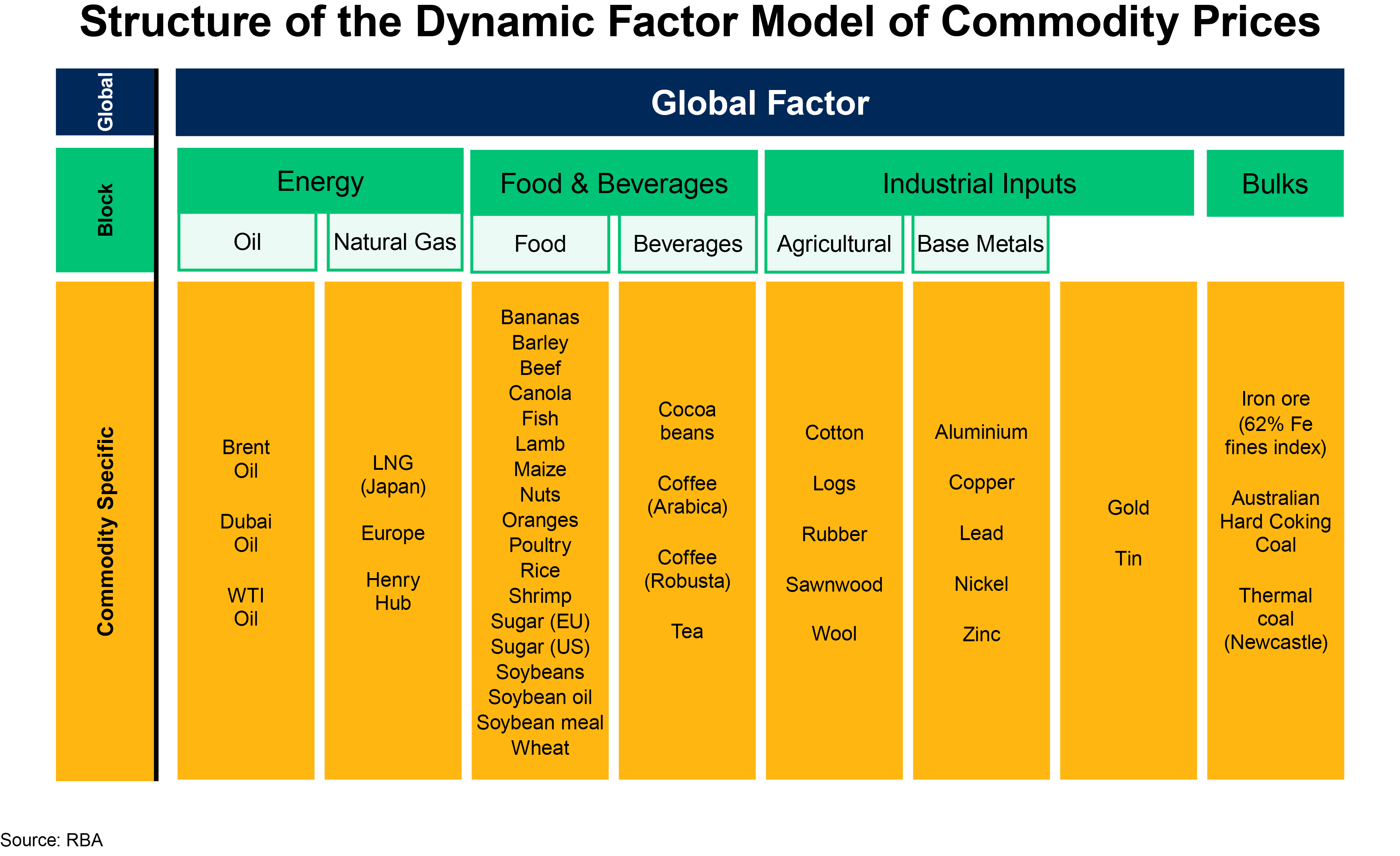
The example of Brent crude oil illustrates the structure of the model:

• Global factor. Common variation between Brent crude oil and all commodity prices, including those in the energy block, is captured by the global factor.
• Block factor. Brent is one of three benchmark oil prices, which all appear in the oil sub-block because they are close substitutes and their prices tend to co-move. The unobserved ‘oil block factor’ captures common variation that is shared between these three prices. Because oil is one of several energy commodities, the three oil prices are then grouped with several natural gas prices under the broader ‘energy block’. The unobserved factor – ‘energy block factor’ – captures co-movement between all oil and natural gas prices; for instance, owing to the use of oil-based pricing mechanisms in some natural gas contracts (Cassidy and Kosev 2015).
• Commodity-specific factor. Any movement in the price of Brent crude oil that is independent of all other commodities is referred to as ‘Brent commodity-specific’.

The grouping of commodities into blocks and sub-blocks in our model largely follows Delle Chiaie et al (2017) with the exception of bulk commodities, where we establish a new block and include coking coal prices. We use month-average spot prices for 43 energy, food and beverage, industrial and bulk commodities that are important for both the global and Australian economies. Data are primarily sourced from the World Bank's Pink Sheet; we replace some series with our preferred price indices (iron ore, thermal coal, beef, lamb and wheat) and include some additional commodities that are important to Australia (coking coal, wool and canola).

While commodity prices within the same block or sub-block are correlated, the commodity-specific shocks are idiosyncratic and do not affect other commodities. For example, the commodity-specific (or idiosyncratic) component of Brent crude oil cannot spill over into the prices of food and beverages. With respect to oil prices, this assumption appears to be somewhat questionable because oil can be an input into the production process of other commodities. However, Baumeister and Kilian (2014) find that pass-through from oil price shocks to the prices of other commodities is limited. Furthermore, the model is fairly robust to misspecification of the cross-correlation among groups of commodities, in part owing to the large number of commodities in each block (Doz, Giannone and Reichlin 2012).

Interpreting the Global, Block and Commodity-specific Factors

The model outlined above is not a structural one; that is, the contributions of supply and demand developments are not directly modelled. Therefore, we should be cautious in mapping the factors to precise supply or demand developments. However, when complemented with knowledge of broader economic and commodity market developments, the model provides a framework through which to interpret price movements.

The global factor captures the co-movement between all of the commodity prices included in our model, and can be thought of as an indicator of global demand. This is because commodities are used in the production of a wide range of goods, demand for which is generally positively correlated with anticipated and realised global activity; the correlation is particularly strong during major downturns and recoveries (Graph 1).^[4] For example, the global factor declined sharply during episodes such as the Asian financial crisis in the late 1990s, the United States downturn in the early 2000s, and the global financial crisis (GFC), and then rebounded strongly after each of these events.

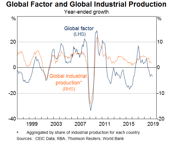
Interpreting the block factors is less straightforward. At any given time, a block factor could capture a change in demand for a specific group of commodities (e.g. Chinese demand for bulk commodities) or a change in supply that is common to that group of commodities (e.g. the largely coincident ramp-up in Australian production of iron ore, coking coal and thermal coal in response to increased demand from China).

The commodity-specific or idiosyncratic component will mainly capture supply factors, because shocks to supply tend to be isolated to one commodity (or a relatively small group of commodities). But demand factors cannot be ruled out – for example, changing regulations or technological advances in the production of a good that affects demand for a specific commodity.

The relative importance of each factor in explaining individual commodity price movements varies across commodities.

• Some commodities have deeper and more liquid futures markets. This means that financial market traders can more readily express their views on the global economy through these markets. Oil and base metals have the deepest and most liquid futures market in our commodity price sample and also display the highest correlation with the global factor.
• China is by far the largest global consumer of most bulk commodities and has consequently had a disproportionate impact on global demand for these commodities. Accordingly, any changes in Chinese demand and government policies tend to have a large influence on bulk commodity prices, which will be mostly captured by the block factor in the model.
• The supply of agricultural commodities can be heavily influenced by weather patterns. Price changes for most agricultural commodities therefore tend to be less correlated with the global factor and have a larger commodity-specific factor that captures these events.
• Some commodities are not easily traded globally and their prices are largely determined in segmented regional markets. The importance of regional developments in determining prices will be captured in either the block or commodity-specific factors of the model, while the global factor will have less of an influence. For example, natural gas markets are regionally segmented and natural gas prices tend to have a low correlation with the global factor.

Applications of the Model

To illustrate the use of the factor model outlined above, we look at some examples of episodes that have been associated with large movements in commodity prices and decompose the price changes into the contributions from the global, block and commodity-specific factors.

The recovery in the price of crude oil between early 2016 and mid 2018

Higher oil prices tend to be associated with an increase in headline inflation; directly through higher automotive fuel prices, and indirectly through the effect that higher oil prices have on the cost of producing goods and services in the economy (see RBA 2015). In recent years, Australia has also shifted from being a net oil importer to a net exporter of oil-price-related products because of the large increase in LNG exports.

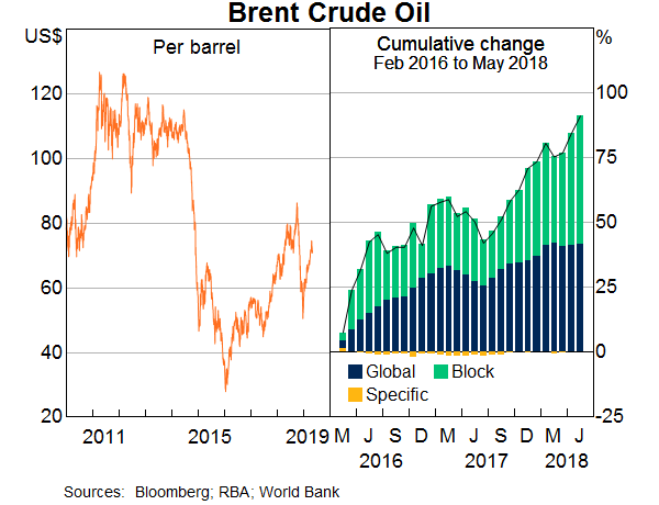
The price of crude oil fell sharply in 2014 and 2015, from over US$110 to a low of US$28 per barrel in January 2016 (Graph 2, left-hand side). The fall in prices followed a large increase in supply of crude oil and natural gas from the United States. This was the result of an increase in the production of ‘unconventional’ oil from new extraction methods (see RBA 2015). Because the growth in production exceeded growth in global crude oil consumption, inventories of crude oil – which are usually fairly stable – rose by nearly 20 per cent.

Oil prices began to recover in early 2016, and more than tripled by around mid 2018. At the time, both demand and supply factors were reported by commentators as supporting the recovery in prices. On the demand side, global economic activity was picking up (see Graph 1 above) and, consistent with this, the outlook for global oil consumption was improving. On the supply side, some oil-exporting economies experienced temporary supply disruptions in 2016, which was then followed by OPEC countries and Russia reaching an agreement to limit production from the beginning of 2017.

Although both supply and demand factors were acknowledged by market analysts as being important for the recovery in crude oil prices, the factor model can help quantify the relative contributions of these effects to the price changes. According to the model, around half of the cumulative increase in the Brent crude oil price can be attributed to the global factor and around half to block factors (Graph 2, right-hand side). The large role of the global factor suggests that the recovery in global industrial production was a significant driver of the rise in the price of Brent crude oil. The block factor is likely to capture supply developments common to oil production, and made an increasing contribution from late 2017 onwards, coinciding with the extension of OPEC-led production cuts through to the end of 2018.^[5]

The increase in bulk commodity prices between mid 2009 and late 2011

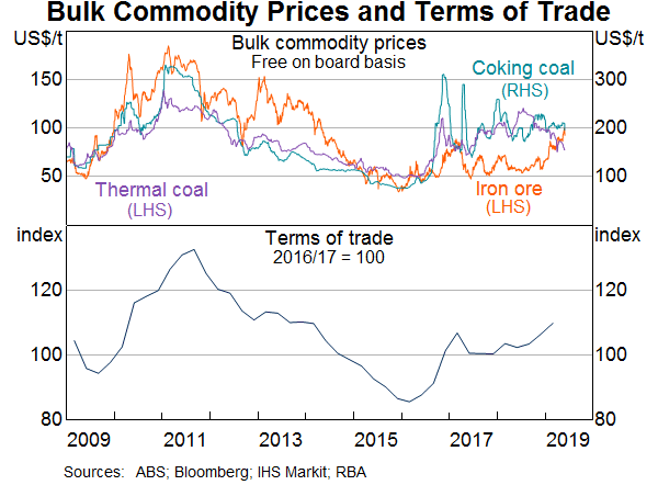
The prices of iron ore, coking coal and thermal coal increased significantly between mid 2009 and late 2011. These increases helped drive Australia's terms of trade and the Australian dollar to historically high levels, and noticeably boosted Australia's national income (Graph 3). The increase in prices for iron ore and coking coal were largely driven by a rebound in global steel production, following the GFC, supported by growth in Chinese steel production (RBA 2010). Strong growth in Chinese steel production – and the associated demand for steelmaking inputs, iron ore and coking coal – was underpinned by Chinese Government stimulus policies that were targeted at infrastructure and construction investment, as well as the ongoing industrialisation and urbanisation of the Chinese economy. Meanwhile, thermal coal prices were supported by increased energy demand needed to support rising global industrial activity.

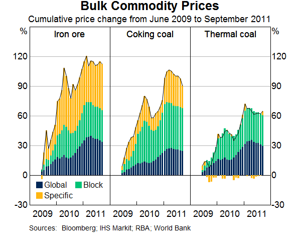
The factor model decomposition provides an additional, and broadly consistent, perspective on the drivers of the price moves between mid 2009 and late 2011. According to the model, the post-financial crisis upswing in global demand, captured by the global factor, accounted for around one-third of the increase in iron ore prices, one-quarter of the increase in coking coal prices, and around half of the increase in thermal coal prices (Graph 4). The block factor accounts for almost half of the increase in coal prices and about one-quarter of the increase in iron ore prices, predominantly capturing the common demand shock from China. While the global and the block factors together accounted for at least half of the increase in the bulk commodities prices over this period, the importance of the commodity-specific factor varied by commodity; it accounted for almost 40 per cent of the increase in the iron ore price, while its contribution to developments in coal prices was smaller. This might reflect a larger increase in Chinese demand for seaborne iron ore compared with coal, because China was able to increase its domestic coal production by considerably more to help meet demand.

In response to the prolonged period of strong, demand-driven price growth, resource companies invested significantly to expand their productive capacity. As these large-scale investment projects have been completed, Australia's exports of bulk commodities, particularly iron ore, have increased considerably.

Tropical Cyclone Debbie and the spike in coking coal prices

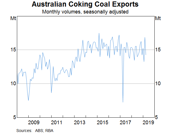
Australia accounts for more than half of the global seaborne coking coal market following the ramp-up in coking coal exports over the past decade. About one-third of Australia's coal exports are produced in the Bowen Basin region in Queensland. Over the past couple of years, there have been some large movements in coking coal prices due to temporary supply disruptions. In April 2017, prices increased sharply after Tropical Cyclone Debbie shut down ports and damaged key rail infrastructure in the Bowen Basin region (Graph 5, left-hand side). The resulting damage to the rail network reduced coal transport capacity over the following month and Australian coking coal exports declined by around 50 per cent in April 2017 (Graph 6). Additional supply-side disruptions in Australia – including temporary mine closures, port congestion and maintenance – in the second half of 2017 also supported prices; however, coking coal prices declined over the early part of 2018 as Australian supply recovered.

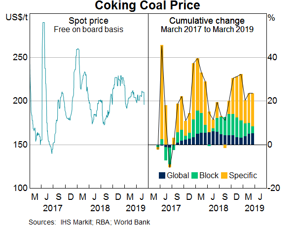
These supply-side disruptions are reflected in the commodity-specific component of the factor model decomposition, which is the primary driver of coking coal price movements over this period (Graph 5, right-hand side). As the seaborne coking coal market is fairly small compared with global production, and Australia accounts for such a large share of seaborne supply, any disruptions to Australian production tends to have a large impact on prices. In contrast, the contributions from the global and block factors were fairly small during this period. Consistent with the transitory nature of the price movement associated with the supply disruption, there was little impact on investment decisions of the major coking coal miners operating Australia.

The impact of recent Australian weather disruptions on the prices of agricultural commodities

Drought conditions across eastern Australia and flooding in northern Queensland have significantly boosted prices of some of Australia's key agricultural commodities, such as wheat and beef. These price movements have also raised some domestic costs and consumer prices, although the effects are likely to be temporary if past experience is any guide.

Wheat prices were also boosted by supply disruptions in other wheat-producing economies, but more recently they have declined as the outlook for northern hemisphere supply has improved (Graph 7, left-hand side). Beef prices initially fell as Australian producers reduced herd sizes in response to the drought, thereby increasing supply (Graph 8, left-hand side). Since their October 2018 lows, however, beef prices have risen by around 35 per cent as the earlier drought-related destocking and flood-related livestock losses have reduced available supply.

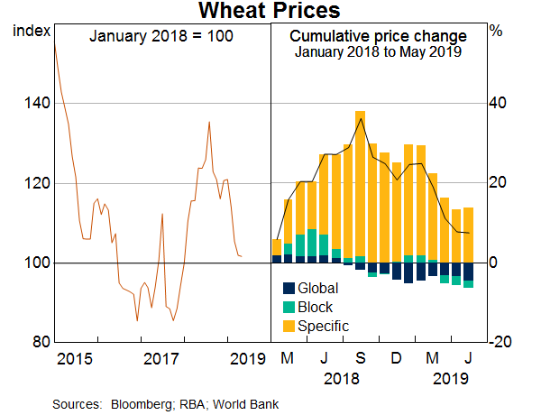
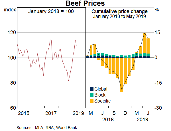
Because the same weather event affects the supply of agricultural commodities in different ways, price movements tend to be driven by the commodity-specific factor (right-hand side of Graph 7 and Graph 8). For wheat, there is a relatively fast reduction in supply following the onset of dry conditions, leading to higher prices; whereas drought-induced herd destocking initially increases beef supply resulting in lower prices, which is then unwound as the impact of reduced supply becomes more of a constraint.

Conclusion

This article decomposes commodity price movements by using a dynamic factor model to estimate the information that is shared between different commodity prices and that which is commodity-specific or idiosyncratic. The relative contributions of global, block and commodity-specific factors to movements in the price of an individual commodity allows us to draw clearer inferences about the relative importance of supply and demand developments to the price change. The factor model will be used to supplement our analysis of commodity price movements, such as in the Statement on Monetary Policy.

Appendix A: A Dynamic Factor Model of Commodity Prices

The (log differenced) price of each of the 43 commodities in our model (listed in Figure 1) is modelled as the sum of $k$ unobservable factors and an idiosyncratic component:

$$x_{it}=c_i{f}_t+e_{it}$$

where $f_t=\left(f_{1t},\dots ,f_{kt}\right)\text{'}$ contains the $k$ global and block factors (see Table A1 for detail on the structure of the blocks in the database) and $c_i={\left(c_{i1},\dots ,c_{i12}\right)}^{\text{'}}$ contains the factor loadings where each element in $c_i$ measures the effect of a global or block factor on commodity $i$ . $c_{ij}=0$ if the commodity is not in factor $j$ .

The factors follow an autoregressive process:

$$f_t=A{f}_{t-1}+{\delta }_t\text{where}{\delta }_t~N\left(0,Q\right)$$

The idiosyncratic or commodity-specific component $$e_{it}$$ also follows an autoregressive process:

$$e_t=\alpha e_{t-1}+{\epsilon }_t\text{where}{\epsilon }_t~N\left(0,R\right)$$

The model is estimated via maximum likelihood, using the Expectation Maximisation algorithm as in Doz et al (2012). First, the algorithm is initialised by computing principal components and using these as estimates of the unobservable factors to then estimate the model parameters using OLS. Second, the estimates of the factors are updated using the Kalman filter. These two steps are iterated until convergence. For more detail see Delle Chiaie et al (2017).

Table A1: Structure of the Commodity Factor Model

Global	Blocks	Sub-blocks	Number of series
All commodities			43
	Energy		6
		Oil	3
		Natural gas	3
	Food & beverages		22
		Food	18
		Beverages	4
	Industrial inputs		12
		Agriculture	5
		Base metals	5
	Bulks		3
Source: Authors' calculations

Footnotes

Michelle Cunningham is from Economic Analysis Department and Emma Smith is from International Department. Alexandra Clarke also contributed to an earlier version of this work while working in Economic Analysis Department. We would like to thank Jarkko Jääskelä, Michelle van der Merwe and Mark Chambers for helpful comments and suggestions, Luke Hartigan for technical assistance, and Reinhard Ellwanger at the Bank of Canada and Simona Delle Chiaie at the European Central Bank for sharing the code used in Delle Chiaie et al (2017). [*]

Other channels via which commodity prices affect the Australia economy are public demand and household expenditure (see Gorajek and Rees 2015). [1]

Similar models are used at other central banks. The model in Delle Chiaie et al (2017) informs commodity price analysis by the ECB, for example Álvarez and Skudelny 2017. The Bank of Canada has adapted the same model for their analysis (Bilgin and Ellwanger, 2017). West and Wong (2014) construct a static factor model of commodity prices, which has been used in research by Wadsworth and Richardson (2017) at the Reserve Bank of New Zealand. [2]

An advantage of the block structure is that by explicitly modelling the local correlation in groups of commodities we avoid over-representation of blocks or sub-blocks with a large number of individual commodities (such as food; Boivin and Ng 2006 and Luciani 2014). [3]

It is possible that the global factor is also being influenced by movements in the US dollar. Commodity prices are generally denominated in US dollars and so they tend to move inversely with changes in the US dollar, thereby keeping the price constant in other currencies. However, results from running the model with commodity prices expressed in special drawing rights (SDR) terms to try and limit the role of the US dollar exchange rate movements suggest that the global factor is not being heavily influenced by US dollar exchange rate movements. [4]

The Brent crude oil specific component, as for the other crude oil prices, makes little contribution to price changes through this period. This is because the prices of different crude oil benchmarks tend to move very closely with each other and, because of their high degree of substitutability, supply developments in different markets tend to impact the prices of all crude oil benchmarks. [5]

References

Álvarez I and F Skudelny (2017), ‘What is driving metal prices?’, ECB Economic Bulletin, Issue 8, pp 36–38.

Baumeister C and L Kilian (2014), ‘Do Oil Prices Increases Cause Higher Food Prices?’, Economic Policy, 80, pp 691–747.

Bilgin D and R Ellwanger (2017), ‘A Dynamic Factor Model for Commodity Prices’, Bank of Canada Staff Analytical Note 2017-12.

Boivin J and S Ng (2006), ‘Are More Data Always Better for Factor Analysis?’, Journal of Econometrics, 127, pp 169–194.

Cassidy N and M Kosev (2015), ‘Australia and the Global LNG Market’, RBA Bulletin, March, pp 33–45.

Chapman B, J Jääskelä and E Smith (2018), ‘A Forward-looking Model of the Australian Dollar’, RBA Bulletin, December, viewed 30 May 2019.

Delle Chiaie S, L Ferrara and D Giannone (2017), ‘Common factors of commodity prices’, ECB Working Paper Series No 2112.

Doz C, D Giannone and L Reichlin (2012), ‘A Quasi-maximum Likelihood Approach for Large, Approximate Dynamic Factor Models’, The Review of Economics and Statistics, 94(4), pp 1014–1024.

Ellis L (2017), ‘The Current Global Expansion’, Australian Business Economists (ABE) Lunchtime Briefing , Sydney, 20 September.

Gorajek A and D Rees (2015), ‘Lower Bulk Commodity Prices and Their Effect on Economic Activity’, RBA Bulletin, September.

Hambur J, L Cockerell, C Potter and M Wright (2015), ‘Modelling the Australian Dollar’, RBA Research Discussion Paper No 12.

Jenner K, A Walker, C Close and T Saunders (2018), ‘Mining Investment Beyond the Boom’, RBA Bulletin, March, viewed 30 May 2019.

Luciani M (2014), ‘Forecasting with Approximate Dynamic Factor Models: The role of non-pervasive shocks’, International Journal of Forecasting, 30, pp 20–29.

Plumb M, C Kent and J Bishop (2013), ‘Implications for the Australian Economy of Strong Growth in Asia’, RBA Research Discussion Paper No 2013-03.

RBA (2010), ‘Box A: The Boom in the Prices of Steel-making Commodities’, RBA Statement on Monetary Policy, May, pp 11–13.

RBA (2015), ‘Box C: The Effects of the Fall in Oil Prices’, RBA Statement on Monetary Policy, February, pp 46–48.

Stevens G (2013), ‘The Australian Dollar: Thirty Years of Floating’, Speech to the Australian Business Economists' Annual Dinner, Sydney, 21 November.

Wadsworth A and A Richardson (2017), ‘A factor model of commodity price co-movements: An application to New Zealand export prices’, RBNZ Analytical Notes AN2017/06.

West K and K-F Wong (2014), ‘A factor model for co-movements of commodity prices’, Journal of International Money and Finance, 42 (April 2014), pp 289–309.