Bulletin – June 2019 Australian Economy Explaining Low Inflation Using Models

Motivation

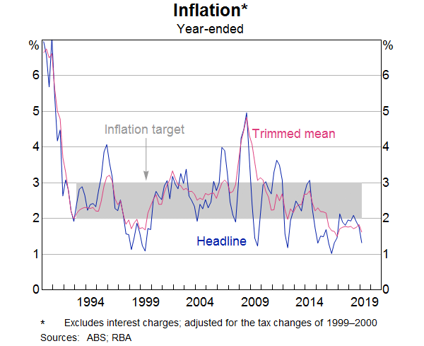
Australia's inflation target is for annual consumer price inflation (CPI) between 2 and 3 per cent, on average, over time (Graph 1). Given the long and variable lags in the transmission of changes in the stance of policy, forecasts for inflation are an important input into the Reserve Bank Board's policy deliberations. Reserve Bank staff employ a range of inflation models to assist in the forecasting process. In recent years, we have made a number of changes to our main inflation models and developed a number of new models. This article explains the choice of variables used to model inflation.

The other motivation for the article is that the inflation models can provide a lens through which to interpret the low inflation outcomes over recent years. The models suggest that spare capacity in the economy is the major reason for these outcomes, while lower inflation expectations have also played a role. More disaggregated models confirm that there has been a broad-based decline in inflationary pressure. Finally, the Reserve Bank's recent inflation forecast performance is discussed.

Inflation Modelling at the Reserve Bank

RBA forecasts reflect our best estimate of future economic outcomes (Kent 2016). This provides a useful starting point to guide policy deliberations and communicate those decisions to the public. The forecasts are published every quarter in the Statement on Monetary Policy.

We employ a suite of single-equation inflation models to provide guidance to the forecasts. We have also recently developed a full-system economic model, known as MARTIN (Cusbert and Kendall 2018) and maintain a dynamic stochastic general equilibrium model (Hambur, Nodari and Gibbs 2018). The difference between single-equation and full-system models is that the former focus on a particular variable (say, inflation) and the variables that explain variations in that variable, such as the unemployment rate, are taken as given. In contrast, full-system models are a system of equations for economic variables that are solved at the same time. The focus of this article is on discussing the set of single-equation inflation models used in forecasting.^[1]

We use a range of inflation models rather than rely upon a single model so that we can incorporate more information into the forecasting process by drawing on a larger set of determinants. It also enables a consistency check across the model forecasts, and may also reduce any bias in the forecasting process. The weight forecasters apply to each of the models in deriving the final forecast for inflation can vary over time.

While the inflation target is defined in terms of headline CPI inflation, the current set of models is designed to explain trimmed mean inflation rather than headline inflation because it is less influenced by volatile and temporary factors. Forecasts for headline CPI inflation tend to be derived by adding on forecasts of volatile items to the trimmed mean forecast. The next section discusses the variables used in the Phillips Curve and Mark-up models of inflation, which are used to forecast aggregate trimmed mean inflation. Following sections discuss a disaggregated model recently developed to explain major components of the CPI basket, known as the Component-level model, and separate models of both tradable and non-tradable inflation.

Aggregate Inflation Models

The two single-equation models that we use to model aggregate inflation are described internally as the Phillips Curve model and the Mark-up model. Earlier versions of these models were detailed in a RBA Research Discussion Paper (Norman and Richards 2010). The structure of both models is guided by theoretical economic relationships, combined with selecting variables based on their statistical performance in the model. Various changes have been made to these models over recent years as more is learnt about the relationships between variables, and as those relationships themselves evolve. The changes to the models over recent years were especially motivated by a desire to improve their forecast performance, and by changes to the way that the Reserve Bank measures some of the input variables used in the models.

The Phillips Curve model estimates a relationship between inflation, a measure of labour market spare capacity and inflation expectations. The following variables are included in the model (and discussed in more detail below):

• The ‘unemployment gap’ – that is, the difference between the unemployment rate and an estimated measure of the non-accelerating inflation rate of unemployment (NAIRU).
• Inflation expectations, because theory suggests that inflation expectations play a role in price-setting behaviour.
• Changes in the prices of imported goods are included, recognising Australia's relatively open economy. Australian consumers and businesses use imported goods and imported goods compete with many domestically produced goods.
• Inflation in the previous quarter, which can be interpreted as representing the component of inflation expectations that is backward looking.

The Mark-up model is based on the theory that firms set their prices as a mark-up over costs. As such, the model includes the following variables:

• Unit labour costs. This is measured as labour costs adjusted for labour productivity gains.
• Changes in the prices of imported goods, motivated in this context by the impact of intermediate imported goods on firm costs.
• Capacity utilisation in the economy. In this model, we use the output gap, which provides a guide to whether economic activity is above or below its (estimated) potential level.^[2]
• Inflation expectations.
• Inflation in the previous quarter.

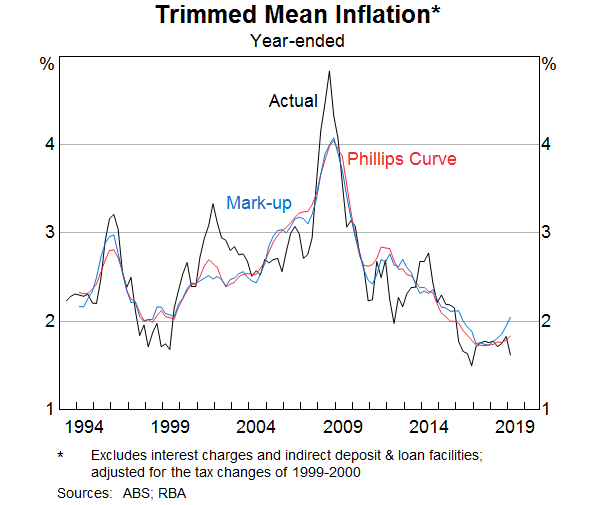
The coefficients of the models are estimated over the period since inflation targeting was introduced. These models fit many of the trend movements of trimmed mean inflation (Graph 2). For instance, both models capture the increase in inflation in the mid 2000s and the decline in inflation since the mid 2010s. The appendix provides the most recent estimated coefficients of the models and their recent performance is discussed in a separate section below.

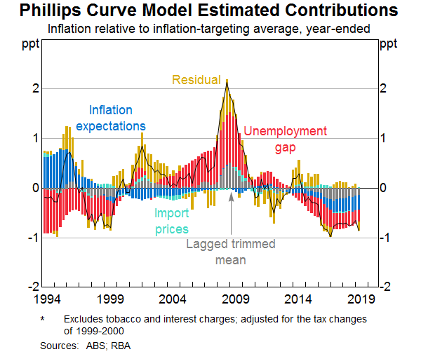
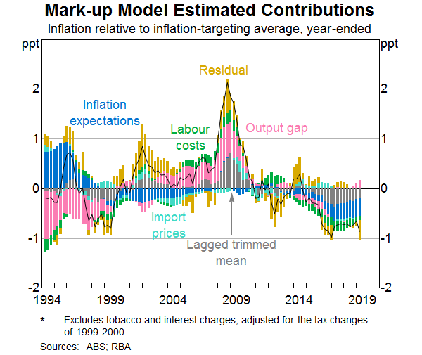
A model decomposition shows the estimated contribution that different variables have made to inflation outcomes since 1993. The stacked bars in Graph 3 and Graph 4 show the contribution each model's input variables makes to the deviation of trimmed mean inflation from its average since 1993. The portion of inflation variance that cannot be explained by the explanatory variables – the model ‘residuals’ – are shown in the gold bars. Some key takeaways from the graphs are:

• The level of spare capacity in the economy (measured as the unemployment gap in the Phillips Curve model and the output gap in the Mark-up model) is an important determinant of inflation outcomes. In both models, variation in the amount of spare capacity can account for around half the variation in trimmed mean inflation when second round effects (via the lagged inflation variable included in the model) are taken into account.^[3]
• During the 2000s, a sustained period of labour market tightness and a positive output gap stoked higher labour cost growth and broader inflationary pressures. However, the models were surprised by the extent of the increase in inflation in 2008, which can be seen in the series of positive residuals during this time.
• Over the past five years, the spare capacity in the economy and associated low wages growth has put downward pressure on inflation. Another source of downward pressure on inflation in recent years has been the decline in inflation expectations. A challenge of quantifying the relative contributions of spare capacity and inflation expectations is that neither are directly observed, and so these explanatory variables must themselves be estimated from the indicators available. Changes in imported prices have had only a small effect recently. While the models were a little surprised by the decline in inflation in 2016, there has been no consistent positive or negative residual more recently.

Spare capacity in the economy

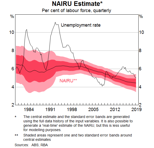
Measures of spare capacity in the economy are important inputs into the inflation forecasts. In the Phillips Curve model, spare capacity is measured as the gap between the unemployment rate and the RBA's central estimate of the NAIRU. The NAIRU is the unemployment rate consistent with stable inflation over the medium term. It is not observable and has to be estimated. Our current approach is to update our NAIRU estimate as we get new data on unemployment, labour costs and inflation based on a Philips Curve framework that treats the NAIRU as an unobserved variable (Cusbert 2017).^[4] The NAIRU is slow moving most of the time and, as such, most of the change in the unemployment gap comes about through changes in the unemployment rate.

There is always considerable uncertainty around the estimate of the NAIRU. The 95 per cent confidence interval around the NAIRU estimate is around ±1 percentage point (Graph 5). The central estimate is also sensitive to the methodology chosen to estimate the NAIRU. There are many alternative ways to estimate the NAIRU, such as using a Hodrick-Prescott filter to extract the trend component in the unemployment rate or modelling the NAIRU as a function of the variables that affect the structure of the labour market. Notwithstanding these caveats, the Reserve Bank's preferred estimate of the NAIRU has declined a little over recent years to be around 4½ per cent.^[5]

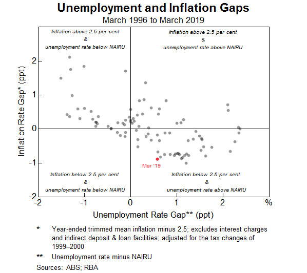
A number of commentators have suggested that the link between inflation and labour market developments has weakened over time.^[6] That is, there is evidence across advanced economies that the coefficient on the unemployment gap in the Phillips Curve has declined, so that inflation would not rise as much as previously when labour markets tighten. The reasons put forward for this ‘flatter’ Phillips Curve include the anchoring of inflation expectations around inflation objectives during the 1990s, increased globalisation of labour and product markets, and changes in the relative bargaining power of labour. At face value, the fact that core measures of inflation in other advanced economies have remained low despite the unemployment rate declining below estimates of the NAIRU, provides some support to this hypothesis. In Australia, the current combination of low inflation and unemployment above the NAIRU is not obviously outside the bounds of historical experience since the mid 1990s (Graph 6). That said, there is some tentative evidence that the slope of the Phillips Curve has declined since the early 1990s, though it is difficult to be certain about the extent of this. There is stronger evidence that inflation has become more stable because inflation expectations have become more strongly anchored (Gillitzer and Simon 2015).

The Mark-up model's measure of spare capacity is the output gap, which measures the deviation of GDP from its potential level. Its influence in the Mark-up model is somewhat smaller than the role of the unemployment gap in the Phillips Curve model. Like the NAIRU, potential output is not observable and has to be estimated. Our primary current method for estimating potential output is based on a ‘production function approach’. This calculates potential output as the weighted average of smoothed growth in the capital stock and labour inputs plus growth in multifactor productivity. There are many techniques for estimating potential output and each method has its strengths and weaknesses.^[7] Notwithstanding this, our output gap estimate suggests the decline in inflation over recent years is consistent with there being spare capacity in the economy (although this spare capacity has gradually declined over recent years).

Inflation expectations

Inflation expectations are understood to play an important role in price-setting and, as such, should contain information about future inflation. Longer-run expectations are also linked to the inflation target, if it is credible. The Reserve Bank monitors a range of survey-based and financial market-based measures of inflation expectations. Each measure has its advantages and disadvantages (Moore 2016). For example, financial market measures such as inflation swaps and inflation-indexed government bonds are useful because market participants have strong financial incentives to estimate future inflation. However, movements in these measures are difficult to interpret because these markets are not particularly liquid in Australia. This means these measures have an embedded, time-varying liquidity premium, and can also contain an inflation risk premium that varies over time to compensate investors for bearing inflation risk. It is also not clear that market participants' expectations affect pricing decisions elsewhere in the economy. Consumer expectations of inflation should also be relevant for inflation dynamics, however, in practice, consumer survey measures do not line up very well with actual future inflation outcomes. Firms set prices but their inflation expectations are not generally surveyed.

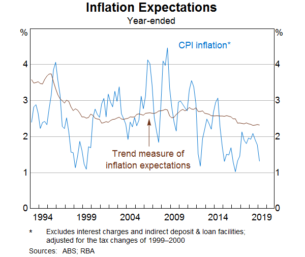
To get around some of these issues, we combine a range of measures of inflation expectations into a single ‘trend’ measure. Specifically, we extract a common signal of expectations from the various measures after controlling for each measure's co-movement with recent inflation (Graph 7). This trend expectations measure is smoother than other series and is a little lower on average because it adjusts for the typical upward bias in many of those individual measures. This is done by adjusting the average of the trend measure to match the average level of the least-biased measures. We treat this measure as a proxy for the inflation expectations of those involved in price-setting in the economy.

Our ‘trend’ measure of inflation expectations, which has an important role in our inflation models, has declined in recent years as a result of fairly broad-based declines in survey and financial market measures of expectations. These declines have been concentrated in the short end of expectations. Gillitzer and Simon (2015) observed that long-term inflation expectations have been firmly anchored since the Reserve Bank adopted an inflation-targeting framework in the 1990s. Consistent with this, long-run survey-based measures of inflation expectations remain around 2.5 per cent.

Labour costs

The inclusion of labour costs in the Mark-up model is based on a view that increases in labour costs in excess of productivity growth (unit labour costs) should put upward pressure on prices because labour costs are the largest component of business costs.^[8] However, in our model, we find that labour costs have only a small role to play in explaining inflation dynamics over the past 25 years. This may be because the measure of unit labour costs in our model is too volatile or mismeasured.^[9] Or it might be because it is difficult to discern an independent effect of changes in labour costs on inflation once spare capacity in the economy (picked up in the output gap) is accounted for.

While we find little evidence of a significant relationship between labour costs and inflation, the fact that price and wage inflation have been low at the same time in Australia and in a range of other advanced economies, provides evidence of some sort of relationship. An ongoing puzzle in Australia is that, in contrast to inflation models, standard Phillips Curve models of wages growth cannot fully explain the weakness in wages growth over recent years.

Import prices

Import prices for consumer goods are included in both the Phillips Curve and Mark-up models because imports account for around one-fifth of the cost structure of final consumer prices in Australia, and many domestically produced goods compete with imported goods. It is also the case that movements in the exchange rate flow through to import prices almost one-for-one. But according to our model, the flow-through from import prices to consumer prices is small. One possible reason is that the models are for trimmed mean inflation, and it may be that CPI components that are heavily influenced by changes in import prices, such as retail goods or fuel, tend to be trimmed out. This provides additional motivation for the development of the tradables model described in the next section.

Disaggregated Inflation Models

While the aggregate models help explain inflation outcomes using only a few variables, there is often a wide range of other factors influencing inflation. Over the years, various disaggregated models of inflation have been constructed by Reserve Bank staff. The models allow us to incorporate idiosyncratic movements in components into the aggregate profile and are also useful for scenario analysis.

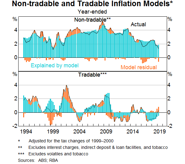
We have developed separate Non-tradable and Tradable inflation models because there have been large differences in inflation outcomes for non-tradable and tradable items over the past two decades. Non-tradable items, which are around two-thirds of the CPI basket, are exposed to a low degree of international competition (such as services that can only be provided locally), and have prices that are influenced more heavily by domestic factors, such as spare capacity in the labour market (Jacobs and Williams 2014). In contrast, tradable items are much more affected by prices set on world markets and fluctuations in the exchange rate, and less influenced by domestic conditions.

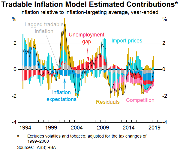
The Non-tradable model is similar to the aggregate Phillips Curve model in that it includes the unemployment gap, a trend inflation expectations measure and its own lag (the appendix provides the details). It also includes a handful of adjustments for government policy changes that have had large one-off effects on non-tradable inflation, such as the introduction of the private health insurance rebate in 1999. Like our aggregate models, the Non-tradable model is unable to fully explain the weakness in inflation in 2015 and 2016 (Graph 8). The Tradable model contains many of the same variables as the Non-tradable model, with the addition of four lags of quarterly import price growth. The coefficients on the import price growth lags suggest that a 1 percentage point increase in import prices leads to year-ended tradable inflation being close to 0.2 percentage point higher over the subsequent year. The model also includes an adjustment to account for the recent period of structural change in the retail industry (see Box).

At a finer level of disaggregation, Reserve Bank staff have also constructed a Component-level model that seeks to explain and forecast a number of expenditure group classifications separately and then aggregates these to construct both headline and trimmed mean inflation forecasts. The groups that are modelled separately include rents, new dwelling costs, tobacco, administered prices, utilities, market services, volatile items, retail items and travel. Some of these groups, such as retail items, are further disaggregated and modelled.^[10] The Component-level models are unable to fully explain the weakness in inflation over 2016 as well as over the past year (Graph 9). The residuals during these periods are predominantly related to prices for administered items and travel.

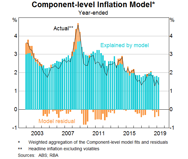
As has been previously noted, slower growth in some administered prices, low increases in rents and competition in the retail sector have all been important contributors to recent low inflation outcomes (Debelle 2018). In the Box below, we single out retail prices to demonstrate the benefits of including disaggregated models in the suite of inflation models monitored.

Forecasting Performance

The decomposition of aggregate inflation in Graphs 3 and 4 demonstrates that a small number of macroeconomic determinants can largely account for the low inflation outcomes over recent years. The bars showing the residuals (or unexplained component) in these graphs indicate that, after the fact, low inflation has not been that surprising given the factors described above (perhaps with the exception of 2016).

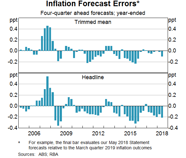
We are also interested in the performance of the RBA's externally published inflation forecasts, which reflect only information available at the time. These forecasts are heavily informed by the models but can also embody a layer of judgement imposed by Reserve Bank staff. Graph 11 shows the forecast errors at the one-year (or four-quarter) horizon; that is, the deviation of actual inflation compared to the forecast one year earlier. The RBA significantly under-predicted inflation outcomes for 2008 and over-predicted future inflation for 2012 and 2015–16. Our forecasts for headline inflation have tended to be less accurate than for underlying inflation. This reflects misses on volatile items which, inherently, are difficult to forecast.

The inflation forecasts that have been published over the past decade do not reflect a consistent set of model forecasts. This is because the updated models outlined in this article have only been in place since late 2016.^[11] Nevertheless, in an assessment of forecast errors, it is helpful to assess the portion of the forecast miss that can be accounted for by errors in the inputs to the models. For instance, it is useful to know whether an inflation forecast error was because of an error in the unemployment rate forecast or other reasons. In 2006 and 2007, the Bank was forecasting the unemployment rate to pick up gradually over the period to 2008. However, the unemployment rate actually declined over this period, contributing to stronger than expected inflation outcomes. The forecast errors in 2015 and 2016 are most likely due to a combination of factors; inflation expectations and wages growth declined by more than expected, while it is also likely that an unanticipated decline in administered prices during this period contributed to the error.

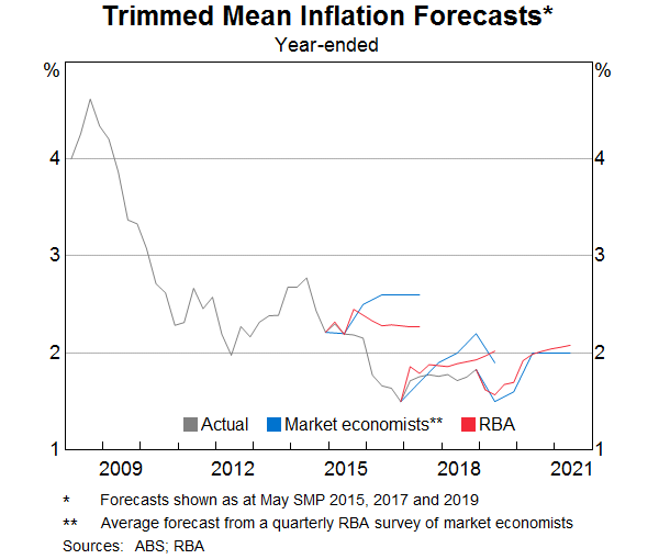
Since the beginning of 2017, the trimmed mean inflation forecasts at a one-year horizon have been relatively accurate. This may be because inflation has been relatively stable over this period. It is too early to judge whether it reflects the impact of improvements made to our modelling framework in 2016. In recent years, the pattern of RBA forecast misses has been broadly similar to the pattern of forecast misses of other professional forecasters (Graph 12).

Conclusion

Year-ended underlying inflation has been around 1½–1¾ per cent for three years, and the RBA's inflation models attribute much of this to a period of spare capacity and low labour cost growth in the economy. The same models underpin a forecast that underlying inflation is expected to rise gradually over the next two years as spare capacity diminishes a little and labour cost growth increases gradually.

Development and refinement of the RBA's inflation models is an ongoing process, as it should be. As new data are released, more is learnt about the behaviour of the Australian economy and how it is changing over time. Several areas of potential improvement are front of mind. While the decline in labour cost growth can explain a sizeable portion of recent low price inflation, labour cost growth has been surprisingly low and hard to fully explain; investigation continues into the relationship between wage and price determination. There is also a stream of research underway looking for a better explanation of the weakness in retail price inflation over the past decade. Work is also ongoing to improve the way we estimate and use ‘unobserved variables’ such as potential output growth, the NAIRU and inflation expectations in our forecasting process.

Appendix: Model Specifications and Coefficients

Table A1: Phillips Curve Model

Estimated on Mar 1993 – Dec 2018^(a)

	Estimate	Standard Error
Intercept	−0.001	(0.126)
${\pi }_{t-1}$	0.211*	(0.094)
$\frac{tren{d}_t}{4}$ (b)	0.808***	(0.206)
$\left(\frac{u_{t-2}-u_{t-2}^{\text{*}}}{u_{t-2}}\right)$ (b)	−0.643***	(0.113)
$\frac{\%{\text{Δ}}^{\text{ye}}(consumerIP{I}_{t-1})}{4}$	0.011	(0.001)
Adjusted R2	0.45
(a) * = 0.05, ** = 0.01, *** = 0.001 (b) The standard errors on these variables are incorrect due to the generated regressors problem.

Table A2: Mark-up Model

Estimated on Mar 1993 – Dec 2018^(a)

	Estimate	Standard Error
Intercept	−0.230	(0.154)
${\pi }_{t-1}$	0.292**	(0.091)
$\frac{tren{d}_t}{4}$ (b)	0.961***	(0.248)
$\left(y_{t-2}-y_{t-2}^{\text{*}}\right)$ (b)	0.054***	(0.014)
$\frac{\%{\text{Δ}}^{\text{ye}}(consumerIP{I}_{t-1})}{4}$	0.021	(0.011)
PDL coefficients on: $\%\text{Δ}\left(NUL{C}_t\right)$
Constant term	0.010	(0.006)
Adjusted R2	0.43
(a) * = 0.05, ** = 0.01, *** = 0.001 (b) The standard errors on these variables are incorrect due to the generated regressors problem.

Table A3: Tradable and Non-tradable Models

Estimated on Mar 1993 – Dec 2018^(a)

	Non-tradable Model		Tradable Model
	Estimate	Standard Error	Estimate	Standard Error
Intercept	0.157	(0.217)	−0.498	(0.317)
${\pi }_{t-1}^{nt}$	0.157	(0.096)
${\pi }_{t-1}^{tr}$			0.059	(0.097)
$\frac{tren{d}_t}{4}$ (b)	0.920**	(0.371)	1.050*	(0.467)
$\left(\frac{u_{t-1}-u_{t-1}^{\text{*}}}{u_{t-1}}\right)$ (b)	−0.890***	(0.215)	−0.368	(0.215)
${\displaystyle \sum }_{j=1}^4{\text{\%Δ}}^{\text{qtr}}consumerIP{I}_{t-j}$ (c)			0.154***	(0.025)
$CompDu{m}_t$			−0.274***	(0.081)
Policy dummies
Health (Sep 1997)	−0.725***	(0.199)
Health (Dec 1997)	0.404	(0.205)
Health (Mar 1999)	−1.081***	(0.199)
GST (Sep 2000)(d)	−0.791***	(0.198)	0.428	(0.313)
Child care (Sep 2007)	−0.286	(0.204)
Child care (Sep 2008)	0.102	(0.204)
Health; Energy (Sep 2012)	0.743***	(0.198)
Energy (Sep 2014)	−0.387	(0.199)
Child care (Sep 2018)	−0.552**	(0.201)
Adjusted R2	0.587	0.471
(a) * = 0.05, ** = 0.01, *** = 0.001 (b) The standard errors on these variables are incorrect due to the generated regressors problem. (c) The estimate provided is the sum of the coefficients on the four lags; joint significance and standard error are determined by a Wald test. (d) There are residual tax-effects in some of the RBA's tax-adjusted CPI data.

Where:

${\pi }_t$	Quarterly trimmed mean inflation (seasonally adjusted), excluding interest charges and indirect deposit & loan facilities; adjusted for the tax changes of 1999-2000.
${\pi }_t^{nt}$	Quarterly non-tradable inflation excluding interest charges and tobacco (seasonally adjusted); adjusted for the tax changes of 1999-2000.
${\pi }_t^{tr}$	Quarterly tradable inflation excluding volatile items and tobacco (seasonally adjusted); adjusted for the tax changes of 1999-2000.
$tren{d}_t$	A measure of trend inflation expectations estimated using a Kalman filter.
$u_t$	The quarterly-average unemployment rate (seasonally adjusted).
$u_t^{\text{*}}$	Non-accelerating inflation rate of unemployment (NAIRU); two-sided smoothed estimate.
${\text{\%Δ}}^{\text{ye}}(consumerIP{I}_t)$	Year-ended growth in the import price index for consumption goods.
${\text{\%Δ}}^{\text{qtr}}(consumerIP{I}_t)$	Quarterly growth in the import price index for consumption goods (seasonally adjusted).
$y_t$	Log non-farm GDP.
$y_t^{\text{*}}$	Log non-farm potential output, estimated using PWL's production function approach.
$\text{\%Δ}(NUL{C}_t)$	Quarterly growth in nominal unit labour costs. The coefficients ${\varphi }_1,\dots ,{\varphi }_{12}$ are assumed to be equal.
$CompDu{m}_t$	A dummy variable with value one from Dec 2010 to present. This accounts for an apparent structural break in the relationship between tradable inflation and the model's explanatory variables, most likely reflecting an intensification in competitive pressures in the retail industry.

Footnotes

The authors are from Economic Analysis Department. The authors would also like to thank Alexander Ballantyne and Martin McCarthy for their valuable contribution in model development over recent years, as well as Angus Moore for his assistance in the forecast performance assessment. [*]

The approach to modelling and forecasting inflation at the RBA has many similarities to the approaches taken at other central banks. For instance, at the Bank of England, a larger ‘structural central organising model’ named COMPASS is run alongside a suite of models with different frameworks including some focused on firm input prices and a ‘bottom-up’ model which projects individual CPI components (Burgess et al 2013). At the Reserve Bank of New Zealand, tradable and non-tradable inflation are modelled separately taking consideration of spare capacity in the economy and movements in the exchange rate (Kergozou and Ranchhod 2013); a structural macroeconomic model named NZSIM models prices as a mark-up over firm's costs (Austin and Reid 2017). [1]

The Reserve Bank has a number of methods for estimating potential output and the output gap, most of which are statistical approaches to filtering out the trend and cyclical components of GDP growth. The output gap is included in addition to unit labour costs in this model to account for the cyclicality of non-wage business costs and mark-ups. [2]

Note that there is negative covariance between the contributions of spare capacity and the contributions of some other explanatory variables in both models. As a result, when this method of variance decomposition is used for each of the explanatory variables individually and these results are aggregated, the total proportion of variance in trimmed mean inflation that the model explains can be overstated. This does not impact the contributions shown in Graphs 3 and 4. [3]

The NAIRU can move in response to persistent shocks to wage and price-setting or variables that are not included in the model. For example, structural change in the retail industry may be causing inflation to be lower than expected. Since we do not account for this in the NAIRU model, the model will ascribe the lower-than-expected inflation to a lower NAIRU. Note that the Bank's NAIRU model has been modified to some degree since Cusbert (2017). [4]

Graph 5 shows the ‘two-sided’ smoothed estimates of the NAIRU. Real-time estimates of the NAIRU, which are also referred to as ‘one-sided’ estimates, are much more volatile and had been higher in recent years than the most recent two-sided estimates. [5]

See for example Borio (2017), International Monetary Fund (2013), and Jordà et al. (2019). [6]

See Schembri (2018) for an overview of the definition and measurement options of potential output. Estimation techniques include either simple statistical models that filter out short-term fluctuations in output growth, or through structural models that rely on theoretical relationships between variables. [7]

There is also likely to be an influence of inflation outcomes on labour costs, which is not explicitly captured in these inflation models. Other multi-equation models maintained by the Reserve Bank can account for these feedback loops. [8]

An alternative approach would be to use growth in the Wage Price Index (WPI); either in addition to unit labour costs or as an alternative variable. Despite being a less volatile series, the WPI is less theoretically appropriate than unit labour costs for inclusion in an inflation equation since the WPI data are only partially adjusted for changes in productivity. Furthermore, the WPI series commences in 1997, whereas we prefer to condition our inflation models over the whole inflation-targeting period. [9]

This classification can differ from the expenditure group classification that the Australian Bureau of Statistics uses, because it is motivated by grouping items that have similar drivers of inflation. [10]

The Reserve Bank regularly reviews and updates its inflation models. In doing so, we recognise that the reduced-form relationships we estimate are not necessarily stable over time, either because the forces impacting the economy can be persistently different at times or because there are structural changes in the way that the economy functions. [11]

References

Austin N and G Reid (2017), ‘NZSIM: A model of the New Zealand economy for forecasting and policy analysis’, Reserve Bank of New Zealand Bulletin, 80(1).

Ballantyne A and S Langcake (2016), ‘Why Has Retail Inflation Been So Low?’ RBA Bulletin, June, pp 9–17.

Borio C (2017), ‘Through the looking glass’, OMFIF City Lecture, London, 22 September.

Burgess S, E Fernandez-Corugedo, C Groth, R Harrison, F Monti, K Theodoridis and M Waldron (2013), ‘The Bank of England's forecasting platform: COMPASS, MAPS, EASE and the suite of models’, Bank of England Working Paper 471.

Carter M (2019), ‘Competition and Profit Margins in the Retail Trade Sector’, RBA Bulletin, June.

Cusbert T (2017), ‘Estimating the NAIRU and the Unemployment Gap’ RBA Bulletin, June, pp 13–22.

Cusbert T and E Kendall (2018), ‘Meet MARTIN, the RBA's New Macroeconomic Model’, RBA Bulletin, March, viewed 7 June 2019.

Debelle G (2018), ‘Low Inflation’, Address at The Economic Society of Australia (QLD) Business Lunch, Brisbane, 22 August.

Gillitzer C and J Simon (2015), ‘Inflation Targeting: A Victim of Its Own Success’, RBA Research Discussion Paper No 2015–09.

Hambur J, G Nodari and CG Gibbs (2018), ‘DSGE Reno: Adding a Housing Block to a Small Open Economy Model’, RBA Research Discussion Paper No 2018–04.

IMF (2013), ‘The Dog That Didn't Bark: Has Inflation Been Muzzled or Was It Just Sleeping?, World Economic Outlook: Hopes, Realities, Risks, World Economic and Financial Surveys, IMF, Washington DC, pp 79–95.

Jacobs D and T Williams (2014), ‘The Determinants of Non-tradables Inflation’, RBA Bulletin, September, pp 27–38.

Jacobs D, D Perera and T Williams (2014), ‘Inflation and the Cost of Living’, RBA Bulletin, March, pp 33–46.

Jordà Ò, C Marti, F Nechio, E Tallman (2019), ‘Inflation: Stress-Testing the Phillips Curve’, FRBSF Economic Letter 2019-05, 11 February.

Kent C (2016), ‘Economic Forecasting at the Reserve Bank of Australia’ Address to the Economic Society of Australia (Hobart), University of Tasmania, 6 April.

Kergozou N and S Ranchhod (2013), ‘Why has inflation in New Zealand been low?’, Reserve Bank of New Zealand Bulletin, 76(3).

Moore A (2016), ‘Measures of Inflation Expectations in Australia’, RBA Bulletin, December, pp 23–31.

Norman D and A Richards (2010), ‘Modelling Inflation in Australia’, RBA Research Discussion Paper No 2010-03.

Schembri LL (2018), ‘The (Mostly) Long and Short of Potential Output’, Speech at the Ottawa Economics Association and CFA Society Ottawa, Ontario, 16 May.