Bulletin – December 2018 Finance A Forward-looking Model of the Australian Dollar
- Download 540KB

Abstract
The exchange rate is an important mechanism that helps the economy adjust to external shocks. This article analyses the key determinants of the Australian dollar – the terms of trade and differences between interest rates in Australia and other advanced economies. It emphasises that ‘forward-looking’ measures of these determinants are important for capturing movements of the observed real exchange rate. In particular, they capture longer-term movements in the real exchange rate, including around key turning points, for instance during the global financial crisis.
The Real Exchange Rate and Its Key Determinants
The Australian dollar was floated in December 1983 and the capital account was liberalised allowing the free movement of capital. Because Australia is a small trade-exposed economy, the flexible exchange rate has been an important buffer against external shocks, particularly during Australia's recent mining investment boom (see Stevens 2013 and Kent 2016). The flexible exchange rate is an important feature of the inflation targeting framework, as it allows monetary policy to respond to domestic economic conditions.
The trade-weighted (TWI) exchange rate is a measure of the Australian dollar against a basket of the currencies of Australia's major trading partners. The Reserve Bank maintains a suite of exchange rate models to help understand movements in the exchange rate. These models are used to assess how consistent the level of the exchange rate is with the level that would be expected based on its historical relationship with other economic variables – or ‘determinants’. These determinants are the terms of trade – the ratio of export to import prices – and prospective investment returns on Australian assets compared with those abroad, commonly captured by real interest rate differentials (Graph 1).
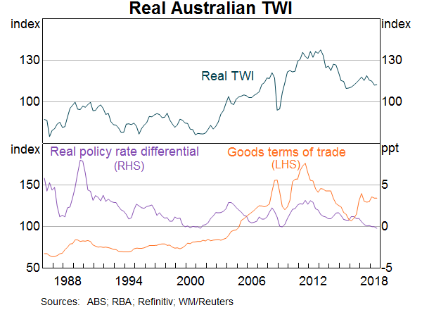
To the extent that participants in financial markets, including foreign exchange markets, are forward looking, expectations about the likely evolution of the economy and a wide range of other relevant variables should be embedded in current prices. Motivated by this, we extend previous work by Hambur et al (2015) by examining whether ‘forward-looking’ measures of both the terms of trade and interest rate differentials exhibit a stronger and more consistent relationship with the real Australian TWI (RTWI) than the observed values of these variables. We restrict ourselves to refining the measurement of these two long-standing determinants, rather than casting the net to include new fundamental drivers.
Our results suggest that deviations of the observed RTWI from its estimated ‘equilibrium’ level over the past three decades are smaller when expectations of the future values of these determinants are used to capture relevant information for the exchange rate.[1] In particular, the RTWI shows relatively small and temporary deviations from the estimated equilibrium around key turning points during the global financial crisis (GFC) and following the peak in the recent mining boom. As these forward-looking determinants capture expectations about the future state of the economy, it is not surprising that the RTWI returns towards its forward-looking equilibrium faster than estimates relying on the current values of the same variables.
Expectations of the Key Determinants of the Exchange Rate
Historically, one of the strongest influences on the Australian RTWI has been the terms of trade (see Stevens 2013 and Hambur et al 2015). However, as market participants are forward looking, there are reasonable grounds to examine whether expected values of the future terms of trade, rather than recent realised outcomes, display a stronger contemporaneous relationship with the RTWI.
Interest rate differentials also matter for the RTWI. One simple, and often used, way to measure interest rate differentials is the spread between the current monetary policy rate in Australia and that of other advanced economies. However, there are many interest rates across different maturities, which collectively comprise the yield curve. The yield curve captures information about the financial market's expectations for the future path of monetary policies, inflation and economic activity.
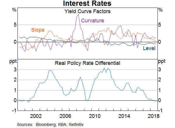
To utilise the forward-looking information embedded across different maturities, the shape of the yield curve can be summarised by three factors: the general ‘level’ of interest rates; the ‘slope’ of the yield curve (the difference between the short- and long-term interest rates); and the ‘curvature’ of the yield curve (Graph 2 provides a stylised presentation of the yield curve; Diebold and Li 2006). Economic literature has shown that these yield curve factors have economic interpretations (although their interpretations may sometimes overlap):[2]
- The ‘level factor’ is associated with inflation expectations.
- The ‘slope factor’ is associated with expectations about inflation, business cycle and economic growth, including uncertainty around the outlook as captured by the ‘term premia’, or the premium received for holding longer-term bonds.
- The ‘curvature factor’ is associated with monetary policy expectations.
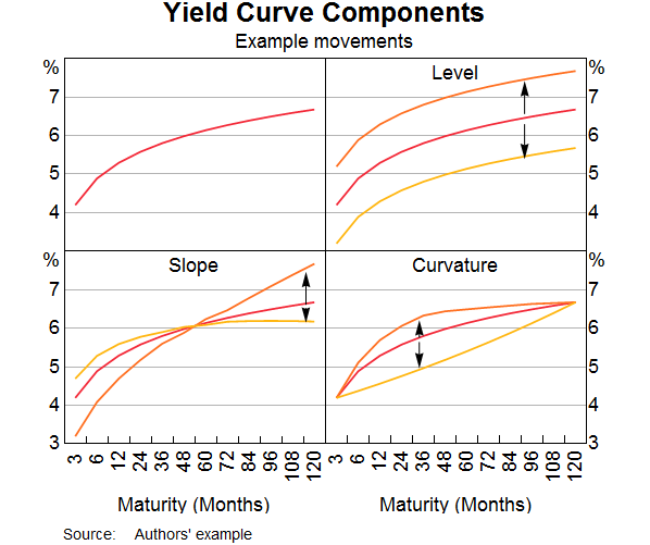
As these yield curve factors are unobservable, they need to be estimated. To do this we use the approach of Nelson and Siegel (1987) (for more details see Appendix A).
A Model of the RTWI
As the equilibrium level of the RTWI is not directly observable, its value must be inferred from the behaviour of the terms of trade, real interest rate differentials and other economic variables. To do this, we estimate the following error correction model (ECM) of the RTWI, which estimates an equilibrium relationship between the (log) RTWI, the (log) terms of trade, and a real interest rate differential:[3]
The ‘speed-of-adjustment’ coefficient (γ) indicates the rate at which the RTWI is expected to return back to this estimated equilibrium when shocks result in temporary deviations.
We consider two alternative sets of the key determinants of the contemporaneous RTWI: ‘current’ (or ‘observed’) values, and ‘forward-looking’ values. The first, ‘baseline’ model uses the current real policy rate differential between Australia and G3 economies (the euro zone, Japan and the United States) and the observed goods terms of trade.[4] The second, ‘forward-looking’ model uses the Reserve Bank's forecasts (two years ahead) for the terms of trade and the three yield curve factors discussed above (level, slope and curvature) in Australia relative to G3 economies as new forward-looking measures of the real interest rate differential. Short-term variables that affect the value of the RTWI – for example, risk sentiment in financial markets (the VIX index) – are also included in both specifications of the model.
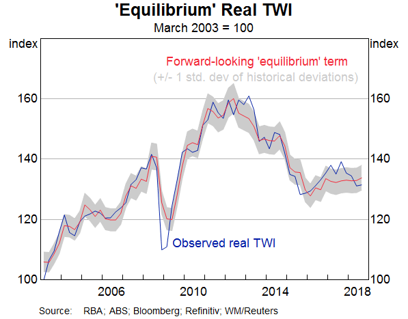
We find that the forward-looking model captures quarterly movements in the RTWI better than the baseline model (Table B1 in Appendix B shows the results obtained when the model is estimated over a quarterly sample from 1986Q3 to 2018Q3). In particular, key turning points in the observed real TWI – for instance, around the GFC and the mining boom – are more closely aligned with the estimated equilibrium level of the forward-looking model when compared to the baseline (Graph 3; these periods are discussed in the next section).[5] Naturally, there are periods when the observed RTWI deviates from its estimated medium-term equilibrium (these are the periods when the RTWI is outside the shaded area in Graph 4, which captures deviations larger than one standard deviation from the estimated equilibrium).
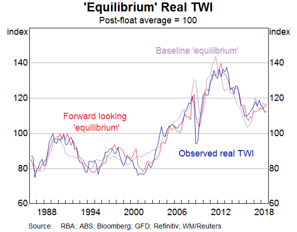
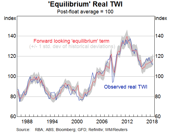
These results suggest that the observed RTWI incorporates expectations of the state of the economy that the baseline model with a single interest differential and current terms of trade does not capture. We find that the yield curve factors are jointly significant (Table B1). In other words, forward-looking foreign exchange markets tend to incorporate expectations on inflation, the business cycle and monetary policy as embedded in the entire yield curve. However, it's not obvious which individual yield curve factor is most important for the RTWI in any given period. Over the sample period, we find that the curvature factor, which has been associated with monetary policy expectations, is statistically significant in the equilibrium relationship. Put differently, expectations for monetary policy appear more important for determining the equilibrium relationship than the current stance of monetary policies. The level factor, which is a proxy for inflation expectations, appears to have a weak relationship with the RTWI over the sample period. Inflation and inflation expectations have generally been low and stable in Australia and the G3 economies over most of the model sample period, so this lack of variation possibly explains the level factor not being a significant determinant of the RTWI.[6]
Finally, the estimation results show that the RTWI returns towards its equilibrium faster in the forward-looking model than estimates relying on the observed values of the same variables in the baseline model. That is, the speed-of-adjustment parameter (γ in the equation above) is larger when the model incorporates expectations on the future state of the economy.[7]
These results appear robust to sample variations
Although the forward-looking model describes movements in the RTWI better than the baseline model, the sample period poses some challenges. First, there has been a substantial change in the macroeconomic environment since the 1980s, including the introduction of inflation targeting in Australia in 1993. Moreover, variables that may have been important for the determination of the exchange rate 30 years ago, for example, the current account deficit, appear less relevant these days. Second, the Reserve Bank's internal terms of trade forecasts are available only from 2003. In order to estimate the model from 1986, we construct forecasts for the terms of trade before 2003. We do this by taking an average of the terms of trade in the previous three quarters (see Appendix B).
It may therefore be preferable to use a shorter sample where genuine terms of trade forecasts are available. In the sample from 2003 onwards, the model explains the quarterly moves in the RTWI more accurately than in the longer, post-1986 sample. As in the post-1986 sample, the yield curve factors are jointly (statistically) significant. However, there are some differences in the importance of the individual yield curve factors across the two sample periods (see Appendix B). For instance, in the short sample, the curvature factor, which is often viewed as a proxy for monetary policy, is not statistically significant in the medium-term equilibrium relationship. This may reflect the lack of relative movement in Australia and G3 policy rates, particularly in the latter part of this period. Rolling regressions (in which the estimated parameters vary over time) do not suggest a high degree of parameter instability and there appears to be no systematic evidence of changes of the speed at which the RTWI reverts back to its estimated equilibrium when it has deviated from it.
Given these considerations, and the fact that the forward-looking model has fitted the observed real exchange rate relatively well in recent years, it is useful to focus on the results of the post-2003 sample period more closely around recent turning points of the RTWI from relatively high levels.
A Closer Look at the Exchange Rate during the GFC and Mining Boom
Accounting for expectations aligns the RTWI more closely with the estimated equilibrium during the GFC and the period following the peak of the mining boom (Graph 5). It is worth considering these episodes in more detail.
The GFC
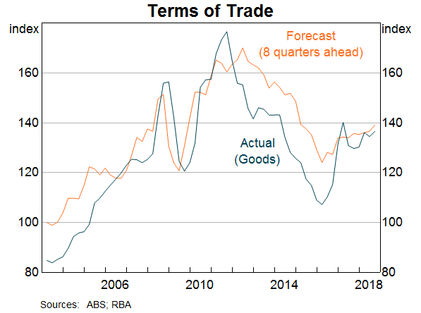
The Australian dollar fell sharply during the GFC. The forward-looking model captures the level of the RTWI and the timing of its subsequent depreciation more accurately than the baseline model. This reflects the fact that the terms of trade was forecast to decline while the actual terms of trade remained elevated (Graph 6). The forward-looking model also captures expectations of easier monetary policy (in the curvature factor) before the real policy rate differential actually started declining (Graph 7). However, the realised depreciation of the RTWI during this period was still more rapid and larger than the model's prediction and, indeed, the trough in the RTWI is well below the estimated medium-term equilibrium. To a large extent, this reflects short-term factors, such as heightened level of risk aversion during the GFC and strains in global funding markets, which are not captured by the medium-term equilibrium value of the RTWI.
The end of the mining boom
The Australian dollar depreciated following the peak in the mining investment boom in 2013. A notable feature of this episode was that the terms of trade began declining about 18 months before the RTWI. The decline in the terms of trade occurred sooner than anticipated; at the time, the terms of trade forecasts remained elevated (Kent 2016). As the timing of the moves in the observed RTWI and the forecast terms of trade align with each other, the forward-looking model captures moves around this period well.
The extraordinary monetary policy measures undertaken in the G3 economies were also likely to have supported the Australian dollar in this period. These policies depressed returns on low-risk assets, such as government debt, encouraging investors to search for investment opportunities that offered a higher yield (the so-called ‘search for yield’). In the low interest rate environment, demand for Australian assets increased. In part, this reflected Australia's creditworthiness (see Stevens 2013).
The forward-looking model captures some aspects of the unconventional nature of monetary policies over this period. The impact of purchases of government securities by central banks is captured in the slope factor, as these purchases pushed down longer-term interest rates. Expectations that policy rates would be kept at low levels for a substantial period of time (as a result of ‘forward guidance’) are captured in the curvature factor.
Conclusions
In this article, we have analysed the key determinants of the real Australian exchange rate – the terms of trade and real interest rate differentials. Forward-looking measures of these determinants appear to be important for explaining movements of the observed real exchange rate. When these are taken into account, deviations of the observed RTWI from its estimated equilibrium level over the recent history were shown to be smaller than when relying on the observed values of the same variables. The real exchange rate shows relatively smaller deviations from the estimated medium-term equilibrium around key turning points, such as during the GFC and following the peak in the recent mining investment boom. However, these historical relationships may not hold in the future.
Appendix A: Estimating the Yield Curve Factors
The approach of Nelson and Siegel (1987) allows us to decompose a yield curve into level, slope and curvature components as follows:
where is the zero-coupon nominal yield on an m-month bond at time t; parameter λ controls the speed of exponential decay, following the convention in literature we set it to 0.0609. The three yield curve factors, level, slope and curvature, are obtained by ordinary least squares estimation for each quarterly observation (t) over the two sample periods (2013 to present and 1986 to present).
Appendix B: Estimating the Forward-looking RTWI Model
The error correction model (ECM) of the RTWI with the relative yield curve factors and forecast terms of trade (ToT) is:
where γ is the speed-of-adjustment coefficient. The model is estimated from 1986 Q3 to 2018 Q3. To calculate the equilibrium level consistent with the medium-term determinants, the short-term variables (i.e. those outside the cointegrating medium-term relationship) are held at their average over the sample.
In order to extend the model sample to 1986 we construct several ‘naive’ estimates of the terms of trade to supplement to the RBA's forecasts of the terms of trade prior to 2003. These naive estimates are an average of the previous three quarters' terms of trade:[8]
| 1986Q3 – 2018Q3 | 2003Q1 – 2018Q3 | ||||
|---|---|---|---|---|---|
| Baseline | Forward-looking | Baseline | Forward-looking | ||
| Constant | 0.42*** | 0.17** | 0.58*** | 0.93*** | |
| Speed-of-adjustment | -0.21*** | -0.34*** | -0.22*** | -0.60*** | |
| Equilibrium relationships | |||||
| Goods ToT | 0.60*** | - | 0.46*** | - | |
| Eight-quarter-ahead forecast ToT | - | 0.90*** | - | 0.68*** | |
| Real policy rate differential | 1.54* | - | 1.93 | - | |
| Level factor | - | -1.56 | - | -0.46 | |
| Slope factor | - | -0.06 | - | 1.37*** | |
| Curvature factor | - | -0.81** | - | 0.06 | |
| Short-run relationships | |||||
| Change in CRB | 0.20*** | 0.19*** | 0.15*** | 0.09* | |
| Change in lagged CRB | -0.03 | -0.03 | -0.01 | 0.01 | |
| Change in S&P500 (SPX) | 0.15** | 0.06 | 0.23*** | 0.17** | |
| Change in VIX | -0.00*** | -0.00** | -0.00** | -0.00* | |
| Change in lagged RTWI | 0.17** | 0.16* | 0.04 | 0.11 | |
| Change in goods ToT | 0.09 | - | 0.00 | - | |
| Change in eight-quarter-ahead forecast ToT | - | 0.45*** | - | 0.35*** | |
| Change in real policy rate differential | 0.06 | - | 2.18** | - | |
| Change in level factor | - | -0.57 | - | 5.16*** | |
| Change in slope factor | - | -0.04 | - | 1.44** | |
| Change in curvature factor | - | -0.39* | - | 0.99*** | |
| Adjusted R2 | 0.48 | 0.49 | 0.77 | 0.85 | |
|
Joint significance Wald test H0: Slope factor = level factor = curvature factor = 0 |
- | p=0.07 | - | p=0.01 | |
|
(a) ***. ** and * indicate statistical significance at the 1, 5 and 10 per cent significance level. Source: Authors' calculations |
|||||
Footnotes
Jarkko Jääskelä and Emma Smith are from International Department and Blair Chapman completed this work in International Department. [*]
The equilibrium level of any exchange rate is not directly observable, but must be inferred from theory or observed variables and relationships. In this article, we model the RTWI based on the observed values of relevant variables. These relationships may not be consistent with theoretical models. Furthermore, as these relationships can change over time, it is difficult to estimate the equilibrium exchange rate precisely. [1]
See Chen and Tsang (2013) for a discussion on using yield curve factors as proxies for market expectations of movements in economic fundamentals. Mishkin (1990a, 1990b) finds the term structure contains information about future inflation. Bekaert, Cho and Moreno (2010) show that inflation is associated with changes in the level factor and monetary policy is associated with variation in the slope and curvature factors. Ang, Piazzesi and Wei (2006) find that the slope of the yield curve can forecast GDP growth. Bui and Fisher (2016) show that the curvature factor is associated with the stance of monetary policy. [2]
First, we perform tests which confirm the necessary conditions for the error correction formulation are met, that is, the RTWI, terms of trade and yield curve factors are non-stationary, integrated of the same order and cointegrated. Augmented Dickey-Fuller (ADF) tests fail to reject the null hypothesis of a unit root in the RTWI, terms of trade and the yield curve factors over most sample periods. A cointegration bounds test (Pesaran, Shin and Smith 2001) indicates that these series are cointegrated. [3]
The goods terms of trade is used in the baseline ECM due to concerns over endogeneity between the RTWI and the services terms of trade (see Stone et al (2005) for details). However, this potential endogeneity problem will not be an issue when using forecasts for the terms of trade given that these forecasts are determined before the RTWI is known. [4]
This conclusion holds in an out-of-sample exercise where the model is estimated up to the peak(s) of the RTWI (2008Q2 and 2013Q1). From thereafter the estimated coefficients are kept fixed and the model is fed with the terms of trade forecasts and the yield curve factors in subsequent quarters. Because the signs of the estimated coefficients do not change between the samples, the estimated equilibrium appears fairly robust to the exclusion (or inclusion) of large changes in the RTWI. [5]
This is also consistent with the idea that differences in rate of inflation between countries matter more for nominal exchange rates than for real exchange rates. The theory of purchasing power parity (PPP) suggests that the nominal exchange rate between two countries will adjust to ensure that purchasing power is equalised in both countries. [6]
Previous work (Hambur et al 2015) similarly found that forecasts of the terms of trade increased the speed of adjustment of the model. [7]
We also considered other naive forecasts, which had lower explanatory power:
Average of previous seven quarters:
Current terms of trade:
[8]
References
Ang A, M Piazzesi and M Wei (2006), ‘What does the yield curve tell us about GDP growth?’, Journal of Econometrics, 131, pp 359–403.
Bekaert G, S Cho and A Moreno (2010), ‘New Keynesian Macroeconomics and the Term Structure’, Journal of Money, Credit and Banking, 42(1), pp 33–62.
Bui AT and LA Fisher (2016), ‘The relative term structure and the Australia-US exchange rate’, Studies in Economics and Finance, 33(3), pp 417–436.
Chen Y-c and KP Tsang (2013), ‘What does the yield curve tell us about exchange rate predictability?’, Review of Economics and Statistics, 95(1), pp 185–205.
Diebold FX and C Li (2006), ‘Forecasting the term structure of government bond yields’, Journal of Econometrics, 130, pp 337–364.
Hambur J, L Cockerell, C Potter, P Smith and M Wright (2015), ‘Modelling the Australian Dollar’, RBA Research Discussion Paper No 2015-12.
Kent C (2016), ‘After the Boom’, Speech at Bloomberg Breakfast, Sydney, 13 September.
Mishkin FS (1990), ‘The Information in the Longer Maturity Term Structure about Future Inflation’, The Quarterly Journal of Economics, 105(3), pp 815–828.
Mishkin FS (1990), ‘What Does the Term Structure Tell Us about Future Inflation?’, Journal of Monetary Economics, 25, pp 77–95.
Nelson CR and AF Siegel (1987), ‘Parsimonious Modelling of Yield Curves’, The Journal of Business, 60(4), pp 473–489.
Pesaran MH, Y Shin and RJ Smith (2001), ‘Bounds testing approaches to the analysis of level relationships’, Journal of Applied Econometrics, 16, pp 289–326.
Stevens G (2013), ‘The Australian Dollar: Thirty Years of Floating’, Speech to the Australian Business Economists’ Annual Dinner, Sydney, 21 November.
Stone A, T Wheatley and L Wilkinson (2005), ‘A Small Model of the Australian Macroeconomy: An Update’, RBA Research Discussion Paper No 2005-11.