RDP 2017-06: Uncertainty and Monetary Policy in Good and Bad Times Appendix B: Robustness Analysis
October 2017
B.1 Identification of Uncertainty Shocks
We test the robustness of our results to three different uncertainty proxies. First, we construct an uncertainty dummy by considering just 10 out of 16 extreme realisations of the VXO, that is, those that are associated to terror, war, or oil events.[26] Second, we identify an uncertainty shock as an unpredictable movement of the VXO itself, obtained via a Cholesky decomposition of the variance-covariance matrix of the estimated VAR residuals. In this exercise, the VXO replaces the uncertainty dummy in the vector of variables we model. Third, we compute an ‘extreme event dummy’ by following the same identification strategy presented in Section 2, but considering the one-month ahead financial uncertainty indicator recently developed by Ludvigson et al (2015). Figure B1 plots the impulse responses of industrial production and employment conditional on these alternative indicators of uncertainty, and contrasts such responses with the baseline results, which turn out to be robust.
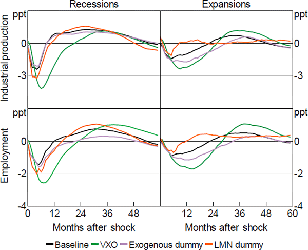
Notes: ‘Baseline’ is the uncertainty dummy as described in the paper; ‘VXO’ is the uncertainty shock identified as the orthogonalised residual of the of the VXO in the VAR; ‘Exogenous dummy’ is the uncertainty dummy constructed by considering extreme realisations of the VXO index related to terror, war and oil events only; ‘LMN dummy’ is the uncertainty dummy constructed by considering extreme events as defined in the paper and associated to the financial uncertainty indicator à la Ludvigson, Ma and Ng (2015)
B.2 Different Calibrations of the Smoothness Parameter
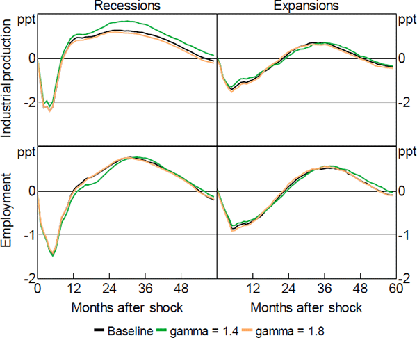
One potential drawback of our empirical exercise is that the smoothness parameter γ of the logistic function of our STVAR, which drives the smoothness with which the economy switches from one regime to another, is calibrated. Our baseline estimation uses a value of γ = 1.8, selected so that the economy spends 14 per cent of the time in recessions (the frequency observed in our sample according to the NBER definition of recessions). To ensure that our results are robust to different values of γ, we re-estimate the model using values of between 1.4 and 2.2, which imply a frequency of recessions in the sample equal to 10 and 25 per cent, respectively. Following Hansen (1999), we set to 10 per cent the frequency corresponding to the minimum amount of observations each regime should contain to be identified. Figure B2 shows the results of this robustness check.
B.3 Unemployment as Transition Indicator
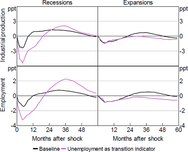
In our baseline exercise, we use industrial production as our transition indicator z. An alternative indicator of the business cycle often considered by policymakers and academics is the unemployment rate. We check the robustness of our results by using the unemployment rate as the transition indicator. Following Ramey and Zubairy (forthcoming), we classify periods in which the unemployment rate is over (under) 6.5 per cent as recessionary (expansionary). We calibrate the smoothness parameter γ = 1.7 to match the 14 per cent frequency of recessions in the sample, as classified by the NBER. Figure B3 documents our GIRFs, which deliver the same stylised facts as in our baseline analysis.
B.4 Uncertainty and Financial Risk
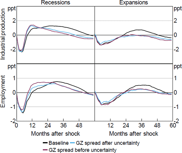
Stock and Watson (2012) point out that financial strains lead to higher uncertainty, which in turn increases financial risk. An implication of this relationship for our analysis is that the transmission of uncertainty shocks may be driven by the level of financial stress in the economy. Caldara et al (2016) provide empirical evidence in favour of larger real effects of uncertainty shocks in periods of high financial stress. A way to control for the presence of time-varying financial risk is by including a measure of credit spread in our VAR. Gilchrist and Zakrajšek (2012) constructed a credit spread cleaned by the systematic movements in default risk of individual firms, the GZ spread. This measure has the attractive feature of isolating the cyclical changes in the relationship between measured default risk and credit spreads. The GZ spread is available from 1973. Our baseline analysis starts in 1962. So we regress the GZ spread against the difference between i) the AAA corporate bonds and the 10-year Treasury yield; ii) the BAA corporate bonds and the 10-year Treasury yield; iii) the 6-month Treasury bill rate and the 3-month Treasury bill rate; iv) the 1-year Treasury yield and the 3-month Treasury bill rate; v) the 10-year Treasury yield and the 3-month Treasury bill rate. We do this for the sample 1973–2008, and then we use the fitted values of the regression to backcast the GZ spread and match our baseline sample. All data are taken from the Federal Reserve Bank of St. Louis' FRED database. We then add this measure of credit spread to our baseline model.
Figure B4 reports the results of this robustness check. We consider two alternative Cholesky orderings to identify uncertainty shocks. First, the credit spread is ordered before uncertainty, implying that uncertainty responds contemporaneously to credit spread but not vice versa. Second, the credit spread is ordered after uncertainty, so to admit a contemporaneous reaction of credit spread to changes in uncertainty. Our results broadly confirm those of our baseline scenario, and are consistent with the findings by Bekaert et al (2013), which show that uncertainty shocks induce business cycle fluctuations even when controlling for indicators of time-varying risk aversion. Our results are also consistent with those in Caldara et al (2016), who show that uncertainty shocks working via credit frictions may lead to a persistent decline in real and financial variables.
B.5 Uncertainty and Housing
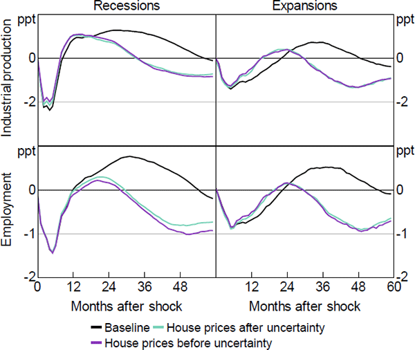
Furlanetto et al (2014) show that uncertainty shocks may play a minor role if one controls for housing shocks. To ensure that our results are not driven by dynamics in the housing market, we add the real home price index computed by Robert Shiller to our baseline model.[27] As before, we consider two alternative orderings and place house prices before and after uncertainty. Figure B5 shows the results of this check. Quite interestingly, the presence of house prices does not appear to affect the drop and rebound of industrial production and employment in bad times. However, it clearly dampens their overshoot in the medium run. In expansions, house prices moderate the response of real activity also in the short run, consistent with Furlanetto et al (2014). However, even when controlling for house prices, we find asymmetric responses of industrial production and employment (in terms of severity of the recession, speed of the recovery, and overall dynamics) over the business cycle.
B.6 Short- versus Long-term Interest Rates
The differences documented in Figure 6 are attributed to different policies as captured by different paths of the federal funds rate. As recalled by Bernanke (2013), however, monetary policy works mainly through the term structure, and in particular via long-term interest rates. Gürkaynak, Sack and Swanson (2005) argue that the Federal Reserve has increasingly relied on communication to affect agents' expectations on long-term rates. In the context of a New-Keynesian framework featuring a term structure of interest rates, Kulish (2007) shows that long-term rates may effectively help in stabilising inflation. Following Bagliano and Favero (1998), we then enrich our VAR with the 10-year Treasury constant maturity rate (ordered after the uncertainty dummy), and re-run our estimates. We run two counterfactuals using this augmented model. The first counterfactual focuses on the response of real activity conditional on a fixed path of the federal funds rate. The aim of this counterfactual is to assess the role of systematic monetary policy when expectations about future rates, as captured by the 10-year rate, are allowed to change. In the second counterfactual, we estimate the responses to an uncertainty shock conditional on a fixed path of the long-term interest rate, that is, under the assumption that expectations about the future stance of monetary policy remain unchanged. This exercise is intended to capture the role that the 10-year rate plays in transmitting the effects of uncertainty shocks. Clearly, the 10-year rate is a combination of expectations over future monetary policy moves and the risk premium, and as such should be considered only as an imperfect proxy of expectations.
Figure B6 plots the impulse responses. Three results stand out. First, the presence of the long-term interest rate does not exert any appreciable impact on the impulse responses, which are very similar to those obtained with our baseline STVAR (shown in Figure 3). This holds true regardless of whether the economy is in a recession or in an expansion. Second, the absence of systematic policy reaction delivers a deeper recession than that predicted by our baseline exercise, even when controlling for the role of expectations about future monetary policy. However, relative to our baseline, the counterfactual recession in this case is milder. In particular, after an uncertainty shock hitting the economy in bad times, real activity returns quicker to steady state relative to the baseline case. This happens because of the role played by the long-term interest rate (possibly via changes in expectations over future monetary policy moves). A third message arising from this exercise is that shutting down the long-rate channel implies that uncertainty shocks hitting in recessions trigger a slower and less marked medium-run recovery (relative to the baseline model augmented with the long-term interest rate). The effect is even more pronounced when uncertainty shocks hit in good times.
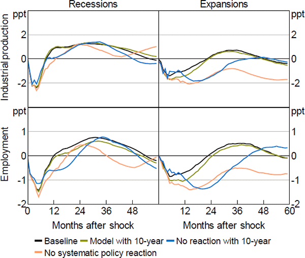
Our results suggest that the long-end of the term structure has important information to understand the effects of an unexpected increase in volatility when the economy experiences a boom. Interestingly, the two channels through which monetary policy may dampen the contractionary effects of uncertainty shocks seem to play a similar role, especially during recessions. Shutting down the short-term rate, which captures systematic monetary policy, or the long-term interest rate, which captures expectations about future monetary policy stance as well as the risk premium, appears to produce similar responses of industrial production in recessions during the first 18 months. Some differences, however, arise when we look at good times. In this case, the role of the long-term interest rate seems to be less important, while the federal funds rate matters much more. The opposite holds for employment, which turns out to be mainly affected by the long-term interest rate. Interestingly, the effects of these counterfactual policies are again larger, especially for expansions, in the medium run, but remain weak in the short run, particularly during recessions.[28]
B.7 Comparison with Linear VAR
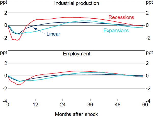
Figure B7 plots the estimated dynamic responses of industrial production and employment to an uncertainty shock obtained with a linear VAR, as well as those conditional on recessions and expansions estimated by our STVAR model. Clearly, a linear model provides a distorted picture of the real effects of uncertainty shocks over the business cycle.
Footnotes
The terror shocks are: the assassination of JFK (November 1963), the 9/11 terrorist attacks (September 2001). The war shocks are: the Cuban missile crisis (October 1962), the Vietnam build-up (August 1966), Cambodia and Kent State (May 1970), Afghanistan and Iran hostages (March 1980), the Gulf War I (October 1990), the Gulf War II (February 2003). The oil shocks are dated December 1973 and November 1978. [26]
The index is available here: <http://www.econ.yale.edu/~shiller/data/Fig2-1.xls> at a quarterly frequency. We moved to monthly frequencies via a cubic interpolation of the quarterly series and modelled the index in logs. [27]
Obviously, caution should be used in interpreting these results, which come from exercises that are subject to the Lucas critique. Ideally, one should build up a model which meaningfully features uncertainty shocks, financial frictions, short- and long-term interest rates, and mechanisms inducing a nonlinear response of real aggregates to uncertainty shocks. We see our results as supporting this research agenda. [28]