RDP 2017-01: Gauging the Uncertainty of the Economic Outlook Using Historical Forecasting Errors: The Federal Reserve's Approach Appendix A

Testing whether Historical Forecasts are Unbiased

Table 7 reports mean errors at horizons 0 to 13, using the sub-samples of forecasters reported in Table 1B. If there are N forecasters in the sub-sample at a specific horizon, the mean at that horizon is

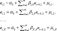
We want to test the hypothesis that for a given horizon is equal to zero, but in doing so we should control for both serial correlation in forecasters' errors plus the correlation of errors across forecasters. To do that, at each horizon we specify the following system of N equations:

In this system, all forecasters are assumed to have the same bias α₀. But we allow their errors to have different degrees of serial correlation (βs). Specifically, for forecast horizons from zero to three quarters, the regression includes the forecasting error at the same horizon for conditions in the previous year. For forecast horizons from four to seven quarters, the regression includes errors at the same horizon for conditions in the previous two years, errors for conditions in the previous three years for horizons from eight to eleven quarters, and errors in the previous four years for horizons greater than eleven quarters. In estimating variance-covariance matrix Ω for the error innovations, μ₁ to μ_N, we allow contemporaneous innovations to be correlated across forecasters and to have different variances. The final step is to estimate this system over the sample period 1996 to 2015, and then to run a standard Wald test by reestimating the system under the restriction that α₀ = 0.

Testing Coverage and Symmetry

To test the likelihood that the observed fraction of errors falling within plus-or-minus one RMSE at a given horizon is insignificantly different from 68 percent, we begin with the same estimated system of equations specified above, with α₀ constrained to equal 0 in all cases. Under the assumption that the error innovations μ₁ to μ_N are distributed normally with mean zero and the estimated historical variance-covariance Ω, we then run 10,000 Monte Carlo simulations to generate a distribution for the number of errors within a 20-year sample period that fall within the designated RMSE band. (Each simulation is run for a 100 year period, and for the test we take results from the last 20 years.) The actual share observed from 1996 to 2015 is then compared to this simulated distribution to determine the likelihood of seeing a share that deviates at least this much from 68 percent, conditional on the true distribution being normal. This same Monte Carlo procedure is used to test whether the observed fraction of errors falling above the RMSE band, less the observed fraction falling below, is statistically different from zero.