RDP 2016-08: The Slowdown in US Productivity Growth: Breaks and Beliefs 2. Model

We work with the model described in Justiniano, Primiceri and Tambalotti (2013). Like other canonical models of the US economy, such as that in Smets and Wouters (2007), this model features a neoclassical core augmented by shocks and frictions that help to explain quarter-to-quarter variation in the data. A desirable feature of the model is that it assumes that TFP growth follows a stochastic trend. A stochastic trend helps the model to account for large and persistent deviations of TFP growth from its steady-state growth rate. This turns out to be important in interpreting the behaviour of the US economy during the 1990s. As the model is standard, we refer readers to Justiniano et al (2013) for a full exposition and Appendix B for the log-linearised equations.

In the model, the growth rate of TFP, z_t , follows the stochastic process:

where γ is the steady-state growth rate of TFP, ρ_z controls the persistence of disturbances to the growth rate of TFP and ε_z,t represent disturbances to the growth rate of TFP. These disturbances follow an independently and identically distributed process with zero mean and constant variance.

2.1 Modelling Structural Breaks in Productivity Growth

In estimation, we allow for breaks in γ, the steady-state growth rate of TFP. We incorporate these breaks using the methods outlined in Kulish and Pagan (forthcoming). In this section we describe the approach when there is a single break in steady-state TFP growth. It is straightforward to generalise the techniques to cases with multiple breaks.

Let t = 1, 2,…, T represent the periods in the data sample. From period t = 1, 2,…, T_γ− 1 steady-state TFP growth takes some initial value, γⁱ. We work with a linear rational expectations model of n equations that can be written as:

where A₀, C₀, A₁, B₀ and D₀ are the structural matrices associated with the initial steady-state TFP growth rate, E_t is the expectations operator, y_t is a n × 1 vector of endogenous variables and ε_t is an l × 1 vector of exogenous variables. We take the latter to be white noise and to have I_ι as their covariance matrix. If a solution to Equation (2) exists and is unique it will be a VAR of the form:

Noting that E_tε_{t + 1} = 0, then if agents know the true structure of the economy it follows that the reduced form coefficients in Equation (3) and structural coefficients in Equation (2) have the relationships:

where .

From t = T_γ, T_γ + 1,…, T, steady-state TFP growth takes some different value, γ^f. The structural form of the model then becomes:

where the superscript * denotes the matrices corresponding to the new TFP growth rate. If agents' beliefs about future TFP growth adjust immediately at T_γ then the solution from this point on is simply , with the reduced form matrices constructed in a similar manner to those in Equations (4)–(6). As well as changing the dynamics of the system, the shift in steady-state productivity growth also changes other steady-state values. This means that even in the perfect foresight case, in which there are no stochastic shocks, a change in steady-state productivity growth will induce transitional dynamics as the economy moves to its new steady state. The technique described above accounts for both the change in the model's steady state and the transition.

We also allow for the possibility that it may take time for agents' beliefs about steady-state TFP growth to adjust to the structural change. In this case there is a period of time in which the actual structure of the economy has altered but agents continue to form expectations based upon the original structure. Formally, let T_b > T_γ denote the date at which beliefs adjust. In the intervening period t = T_γ, T_γ + 1,…, T_b − 1, the actual path of the economy continues to obey Equation (7). However, expectations are based on the initial structure of the economy, that is E_ty_{t + 1} = C + Qy_t. During this time, the solution of the model is given by:

where

and and From t = T_b, T_b + 1,…, T the solution of the model becomes .

2.2 Implications of a Change in Steady-state Productivity Growth

A change in γ alters the growth rate of TFP permanently. In contrast, an innovation to ε_z,t has a temporary (but possibly quite persistent) effect on the growth rate of TFP (although it has a permanent effect on its level). The response of economic variables to temporary and permanent changes in productivity growth differ. This allows us to distinguish between shifts in γ and innovations to ε_z,t in estimation.

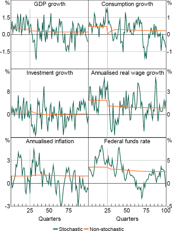
To illustrate this, Figure 2 shows the consequences of a decrease in trend productivity growth for some of the key macroeconomic variables in our model. To construct the figure, we simulate the model for 100 quarters, setting all parameter values except for the one controlling steady-state productivity growth, γ, at the posterior means reported in Justiniano et al (2013). For the first 24 quarters, we set γ equal to 0.50 per cent at a quarterly rate, which is similar to the posterior mean reported in Justiniano et al (2013). In quarter 25, we lower the value of γ by 0.25 percentage points to 0.25. In this example, agents observe the break in steady-state productivity growth when it occurs and adjust their behaviour immediately in response to this change.

In the figure, the lines labelled ‘stochastic’ represent the stochastic simulation of GDP, consumption, investment and real wages growth as well as inflation and interest rates. The lines labelled ‘non-stochastic’ show the non-stochastic path of the variables. This is the path these variables would have followed if the economy experienced no structural shocks but the decrease in steady-state productivity growth still occurred.

Focusing first on the non-stochastic paths, the fall in steady-state productivity growth lowers the growth rate of GDP, consumption and real wages, as expected. The steady-state real interest rate, given by γ/β (where β is the households' intertemporal discount rate), decreases. As the central bank's inflation target remains constant, the steady-state nominal interest rate also falls. It takes a few years for interest rates to reach their steady-state level, however, as the decrease in productivity growth has a modest inflationary impact in the near term.

Perhaps the most surprising response is that of investment growth. This increases in the first few quarters after the break, although it ultimately settles at a lower growth rate. The initial increase in investment growth has two causes. First, on the supply side, the desire of households to reduce consumption in response to an unanticipated fall in productivity growth creates additional savings, which firms can use to invest. Second, on the demand side, the price of new capital falls but overshoots its final level. This creates an incentive for firms to invest in the near term while capital is relatively cheap.

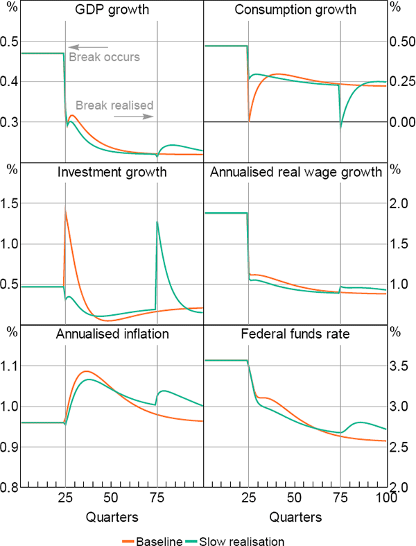
In Figure 2 agents observe the break in productivity growth as it happens. In reality, one might think that agents will take some time to realise that steady-state productivity growth has declined. Figure 3 illustrates the non-stochastic paths of the economy when agents' beliefs do not match reality. In this case, we assume that agents' beliefs about steady-state productivity growth do not adjust until quarter 75, that is, around seven years after the break. For comparison, we also graph the non-stochastic paths from Figure 2 (in which agents observe the change in steady-state productivity growth in real time).

The non-stochastic path of the economy in Figure 3 differs in several respects from that of Figure 2. For example, consumption growth falls when the break in productivity growth occurs and then again when agents' beliefs adjust. The first decrease in consumption is smaller, because households initially anticipate that the fall in productivity growth will be temporary. The second decrease is larger because households realise that productivity growth will be slower permanently. Likewise, investment growth increases when beliefs adjust rather than when the break in productivity growth actually occurs.

Interest rates initially fall by marginally more when agents' beliefs do not adjust immediately. This reflects the fact that the central bank shares the same information set as other agents in the economy. They perceive the slowdown in economic growth to be cyclical rather than structural and accordingly lower interest rates to combat this.

In contrast, most of the slowdown in real wages growth occurs at the time of the break in productivity growth. In the model, despite the presence of nominal wage rigidities, real wages are less forward looking than consumption. Instead, they are more reflective of recent productivity growth outcomes. Consequently, real wages adjust rapidly to a slowdown in trend productivity growth even if agents perceive the slowdown to be transitory.

The simulations in Figures 2 and 3 show that breaks in productivity growth have implications for many observable macroeconomic variables. In estimation, we use these implications to identify the breaks. The simulations also highlight how the response of the economy depends on agents' beliefs about future productivity growth, pointing to the benefits of structural estimation that can take account of these beliefs.

However, comparing the stochastic and non-stochastic paths in Figure 2 also indicates that the quarter-to-quarter volatility in macroeconomic data could be far greater than the dynamics induced by even a relatively large change in steady-state productivity growth. This raises the question of whether our estimation will be able to identify a break in productivity growth successfully. To address this concern, we estimate the parameters of the model using simulated data. We find that we are able to recover the actual parameters with a high degree of accuracy.^[4]

Footnote

Appendix D documents the results of this exercise. [4]