RDP 2019-06: The Effect of Mortgage Debt on Consumer Spending: Evidence from Household-level Data 6. Does Debt Amplify the Effect of Financial Shocks on Spending?
July 2019
- Download the Paper 1,513KB
Next, we explore whether the level of debt makes households more sensitive to other financial shocks (the debt amplifier effect). The debt overhang and debt amplifier effects are intrinsically linked, since financing constraints and uncertainty are likely to be more significant during financial shocks. While this makes it hard to disentangle the debt overhang and amplifier effects, especially at times of large financial shocks, significant debt amplifier effects may provide indirect evidence for the importance of financing constraints and precautionary saving motives in driving the effect of debt on spending.
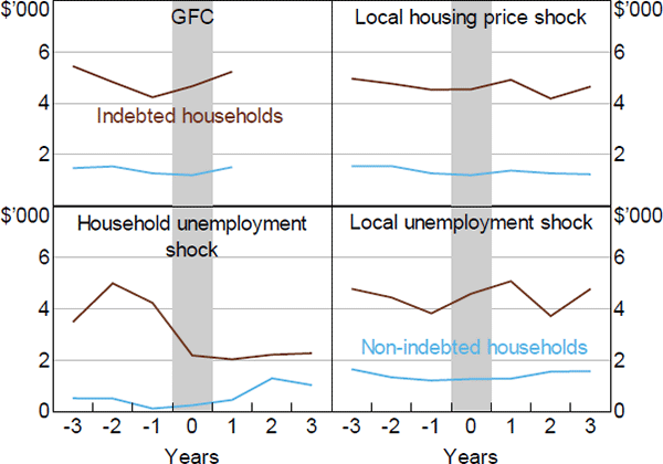
We measure a financial shock in four ways. First, the GFC is used to capture an aggregate shock.[18] Next, we use two measures of a local economic shock: an increase in the regional unemployment rate by more than 1 percentage point in a given year; and a fall in postcode-level housing prices by more than 5 per cent over a year. Finally, we use the household reference person becoming unemployed as a measure of a household-level shock.
If debt makes households more sensitive to shocks, then the spending of highly indebted households should fall by more than the spending of comparable households with lower levels of debt in response to a negative shock. This is precisely what we see in the event of a household unemployment shock (Figure 6).[19] The indebted household reduces its spending on durable goods by more than the non-indebted in the year of the household unemployment shock and spending remains subdued after the shock.[20] In contrast, the effects of the GFC and local economic shocks appear to have been broadly similar across indebted and non-indebted households, although indebted households tend to increase their spending after local economic shocks.

Notes: 2017/18 dollars; households with and without owner-occupier housing debt
Sources: ABS; Authors' calculations; HILDA Survey Release 17.0
While these event studies provide some evidence that debt levels could amplify households' responses to financial shocks, they fail to take into account differences in the characteristics of indebted and non-indebted households, making it unclear whether it is debt per se that is behind the differences in responses. To address this more formally, we add an interaction term between the level of debt and the SHOCK into the FE model. We then test whether the interaction coefficient is significantly different from zero. For example, the FE model is:
Table 7 presents the results for each financial shock. As before, we find a persistent negative and quantitatively similar effect of debt on spending. This suggests that our results for the debt overhang effect are not driven by a higher sensitivity of indebted households to income or wealth shocks alone. We find some evidence for the debt amplifier effect, though it is not present in all specifications.
The debt interaction coefficient is negative for all shocks, but only significantly different from zero for the GFC and the local housing price shocks. These shocks increase the negative effect of debt on spending to around −0.05 or −0.06 per cent. While the event study suggests that households with more debt reduce their spending by more if they become unemployed, the regression estimates do not confirm this. However, even though the interaction effect of debt with household unemployment shocks is negative, it could be imprecisely estimated due to the small sample of survey respondents that have debt and have become unemployed.
| Global financial crisis | Local housing price shock | Household unemployment shock | Local unemployment shock | |
|---|---|---|---|---|
| Lagged mortgage debt | −0.02* (0.07) |
−0.03** (0.03) |
−0.03** (0.01) |
−0.03** (0.04) |
| Lagged mortgage debt × financial shock | −0.03** (0.03) |
−0.03* (0.07) |
−0.13 (0.34) |
−0.02 (0.22) |
| Income | 0.10*** (<0.00) |
0.09*** (<0.00) |
0.09*** (<0.00) |
0.09*** (<0.00) |
| Income × financial shock | <0.00 (0.94) |
0.02 (0.59) |
0.03 (0.92) |
<0.00 (0.88) |
| Lagged home value | 0.11** (0.04) |
0.11** (0.04) |
0.11** (0.04) |
0.10* (0.06) |
| Lagged home value × financial shock | 0.01 (0.64) |
0.01 (0.73) |
−0.23* (0.09) |
0.02 (0.54) |
| Observations | 6,622 | 6,619 | 6,599 | 6,622 |
|
Note: See notes to Table 1 Sources: Authors' calculations; HILDA Survey Release 17.0 |
||||
Footnotes
While the financial crisis began in 2007, the effects of the global recession on Australia were not evident until late 2008. From late 2008 to mid 2009, the unemployment rate increased and salary income fell. The unemployment rate peaked in mid 2009, but remained relatively high for the rest of 2009. Given our focus on households as well as the annual frequency of our data, we define the crisis period as 2009. [18]
Due to small sample sizes for some shocks, in Figure 6 we compare indebted and non-indebted households rather than highly indebted and less-indebted households. [19]
We focus on durables spending in Figure 6 as purchases of durable items are easier to postpone when a shock occurs. However, we find a similar pattern for non-durables spending before and after an unemployment shock. [20]