RDP 2024-10: How Do Global Shocks Affect Australia? 4. How Much Do Global Shocks Affect Australia?
December 2024
- Download the Paper 1.87MB
We now use these estimated factors as the foreign block for our FAVAR. We first assess how much the global shocks captured by these factors matter for variables core to the mandate or toolkit of the RBA. Accordingly, for our domestic block, we use Australian quarterly headline CPI inflation, the (differenced) cash rate and unemployment rate, and (log differenced) nominal TWI and real GDP as a base specification.[13] To formalise the assumption that Australia is a small open economy, we impose that Australian variables do not affect the global factors contemporaneously or with a lag. Imposing these zero restrictions also helps to keep the model parsimonious.
4.1 Evidence from forecast error variance decompositions (FEVDs)
We explore the quantitative importance of global shocks for Australian variables through forecast error variance decompositions (FEVDs). These FEVDs show the sum of variation in our domestic variables that is explained by the global factors relative to the total forecast error variance of the domestic variables (the sum of variation driven by all global and domestic shocks). As is common when conducting inference on impulse response functions (though less common for FEVDs), we construct bootstrapped 68 per cent error bands around the point estimates of the joint contributions of global shocks to the forecast error variance of the domestic variables.[14]
4.1.1 Base specification
Global shocks as captured by our factors have heterogeneous effects on Australian domestic variables (Figure 5). In particular, global shocks appear to explain more variation in the cash rate and the nominal TWI than in headline CPI, real GDP, and, to some extent, the unemployment rate.[15] The finding that variation in the exchange rate and the policy rate is driven to a considerable extent by global shocks is in line with the literature on other small open economies and similar to earlier Australian studies (Jääskelä and Smith 2011; Manalo et al 2014), though the response of other economic variables, particularly GDP, is smaller (e.g. Vasishtha and Maier (2013) for Canada).[16] This observation accords with the notion that the Australian dollar buffers the economy from external shocks (RBA 2020).
These results also accord with the role of monetary policy in buffering the domestic economy from global shocks. Because the RBA targets domestic activity (unemployment) and inflation in line with its mandate, it moves the cash rate to buffer against external shocks that could knock domestic variables off the RBA's preferred path.[17] The nominal TWI appears to adjust to global shocks almost immediately, as seen by global shocks explaining an almost equal share of its variation on impact as at later horizons, in line with the efficient markets hypothesis (Cornell and Dietrich 1978). On the other hand, global shocks appear to feed through more slowly to the cash rate, suggesting these shocks may change the RBA's outlook with a lag, or that the RBA adjusts the cash rate gradually (Lowe and Ellis 1997). To the extent that global shocks could be affecting the RBA's outlook with a lag, this may reflect the fact that it takes time for the nature and size of global shocks to be understood, particularly if the RBA is predominantly responding to the global shock by waiting to see whether the shock affects domestic variables. Further investigating how precisely monetary policy responds to global shocks (and the extent to which policymakers wait to see a domestic effect) is a worthy matter for future research.
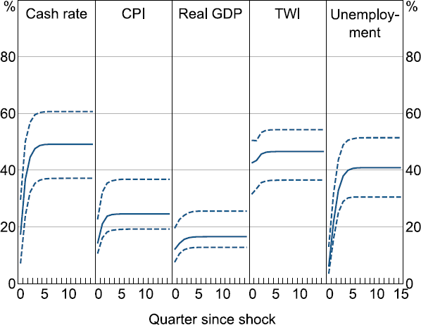
Note: Dashed lines show 68 per cent confidence interval.
A puzzling feature is that global shocks appear to explain significantly more variation in unemployment than in GDP, despite employment being an explicit mandate of the RBA rather than output. Moreover, in an Okun's Law framework, unemployment would be expected to move closely with GDP. One hypothesis is that quarterly real GDP is subject to considerably more measurement error than unemployment (Rees, Lancaster and Finlay 2014), or to temporary idiosyncratic shocks to non-labour-intensive sectors of the economy or sub-components (like non-monetary gold exports, which are highly volatile), and therefore moves less with global shocks than labour market indicators. Moreover, our results are also consistent with prior research that finds a relatively weak relationship between the output gap and the unemployment rate for Australia over our sample period (Lancaster and Tulip 2015).
Another possibility for the greater responsiveness of the labour market relative to output is that the exchange rate and cash rate buffer the Australian economy to remain relatively stable in aggregate, but the substitution of activity between sectors and regions still has noticeable effects on the labour market. This may be best seen through a narrative discussion of key episodes that drive material variation in our factors and the Australian variables. Australian quarterly real GDP growth, which is generally quite noisy, remained relatively stable through the 2001 US recession and the GFC that our first factor picks up as seen in Figure 4. On the other hand, unemployment did tick up in response to each of these episodes (Figure 6). During the GFC for example, the RBA noted that unemployment had risen despite the economy performing better than expected over the year. This coincided with a depreciation in the exchange rate which also brought on some compositional change: the labour markets in Western Australia and Queensland, relatively more mining-exposed and, therefore, export-exposed states, had been strong, while the labour market in New South Wales had deteriorated (RBA 2009a, 2009b).
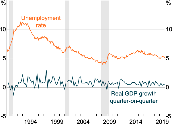
Notes: Seasonally adjusted. Shading indicates US recessions.
Sources: ABS; National Bureau of Economic Research.
Indeed, the mining sector has contributed an increasingly larger share of output, while its share of employment remains relatively low (more than 14 per cent of gross value added against around 2 per cent of employment in 2023). This itself suggests a potential reason that fluctuations in real GDP in recent decades have not been as tightly linked with fluctuations in unemployment as theory would suggest.
Our estimates for the effect of global shocks on GDP are also smaller than prior literature, especially the literature from the 2000s (e.g. Nimark 2007). While some of this may be driven by differences in methods used, it may also be driven by the way shocks originating in the United States are modelled and their changing relevance to Australia. In contrast to this paper, the prior literature almost exclusively studied spillovers from the United States to Australia. We address this issue next.
4.1.2 Comparison to a small-scale VAR
Part of the justification for applying the FAVAR approach in the context of assessing the contribution of global shocks is that it may better span the space of global shocks than a two-country model. We assess this claim by comparing the FEVDs for the base specification of the FAVAR with the results for a small-scale VAR with a foreign block made up solely of US variables.[18] We present the comparison between the FEVD results for the baseline FAVAR and the US foreign block VAR in Figure 7.
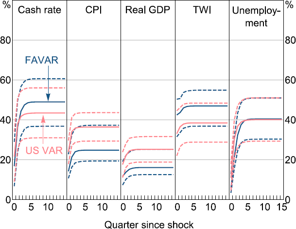
Note: Dashed lines show 68 per cent confidence intervals.
Compared to the small-scale VAR, the FAVAR captures shocks which explain more of the FEV in the cash rate and the TWI, a similar amount of variation in unemployment but less variation in CPI and real GDP, although the difference between the two models does not appear to be statistically significant for any variable. While it appears there are some shocks that the FAVAR is able to capture which a bilateral VAR is not, a US bilateral VAR captures a substantial proportion of the relevant shocks, likely due to the US economy's central importance in the global economy. This does not necessarily mean that the US economy is more important to Australia than the global economy, but it does suggest that variation in US economic and financial variables over 1990–2019 were effectively a ‘sufficient statistic’ for capturing global economic shocks, and indeed possibly better capture global information relevant to Australia's inflation and GDP growth.
4.1.3 Exploring the role of additional factors
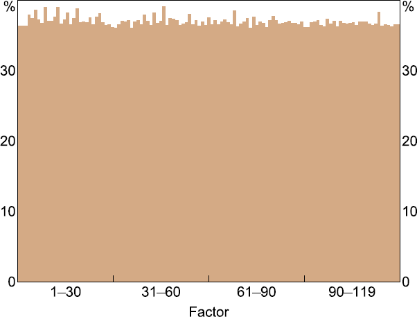
So far, we have estimated the baseline FAVAR using the factors that best explain variation in our panel of global data (this being the purpose of PCA estimation). However, these are not necessarily the same factors that best explain variation in Australian data. We therefore test whether there are other principal components which do not explain variation in the global panel as well, but explain more of the variation in Australian data. To do this we experiment with adding a fourth factor to the baseline FAVAR. We start with the fourth principal component, and then replace that factor one by one with each of the 116 other principal components we calculate, each time assessing the average FEV explained across the Australian variables by all foreign factors when including this particular principal component.
Adding any one of these factors does not explain substantially more variation in the Australian variables than the baseline specification (Figure 8). Regardless, we investigate whether there is some systematic similarity between the excluded factors that explain more variation in Australian variables.
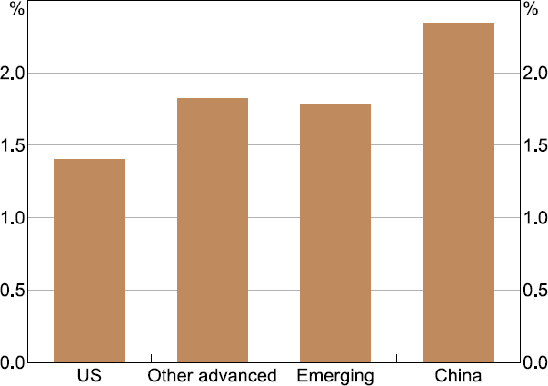
For this, we rank the models shown in Figure 8 and select the five that explain the highest proportion of FEV in the Australian data. These five factors on average explain greater variation in Chinese variables than in variables from other countries (Figure 9). This is unlike the first three principal components we use in the baseline specification, which explain very little variation in Chinese variables (Figure 3).
This suggests that factors that are idiosyncratic to the Chinese economy are more relevant for explaining variation in the Australian economy than explaining variation across the global panel more broadly. This aligns with the particular importance of the Chinese economy to Australia, which comes largely from trade (Guttmann et al 2019). Overall, however, the variation explained in Chinese variables by the alternative fourth factors are relatively low, and the FEV explained by global factors when including the alternative ‘China’ factors is not significantly different from the baseline FEVD.
4.1.4 Are we missing important shocks originating in China?
To test if the low loadings on Chinese variables are leading to lower FEV explained in the Australian data than if we allowed these Chinese variables to directly affect Australian variables, we conduct three further experiments. First, we test a model with the original three factors when estimated on a global panel without any Chinese data. Second, we test a model with the global factors excluding China but explicitly adding four Chinese variables to the foreign block: GDP, industrial production, 10-year government bond yield and CPI. As there may be concerns about measurement error in Chinese GDP data affecting the results, we use the Chinese GDP measure from Barcelona et al (2022), which is generated from a dynamic factor model on a variety of Chinese activity data. Third, we test a bilateral VAR with only the four Chinese variables mentioned alone as the foreign block. We present the FEVDs for the three experiments in Figure 10.
At face value, the results suggest that shocks reflected in Chinese data do not explain material variation in key Australian economic variables. There is little difference between the FEV explained in the Australian data by the model using the factors without China alone and the model with the same factors without China but also including Chinese variables explicitly. The model with the factors without China and additional Chinese variables also explains only marginally more of the variation in the Australian data than the baseline three factors, despite having a considerably richer foreign block. Consistent with that, using the Chinese variables alone explains significantly less of the FEV in Australian variables.
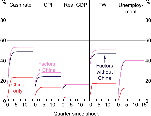
This could suggest that shocks originating in other advanced economies are more important to Australia's economic outcomes than shocks originating from China. On the other hand, Chinese shocks may be just as important for Australia, but shocks originating from China are captured in large part by other global data, while Chinese data are not capturing shocks from other countries. This could be the case for instance if Chinese government policy is explicitly insulating the Chinese economy from global shocks, whereas shocks from the Chinese economy are having observable effects on global data. A third hypothesis is that Chinese shocks are important in explaining the long-run levels of Australian variables, but do not explain substantial short-run variation. Without explicitly identifying the particular shocks, we cannot distinguish between the three hypotheses.
This result may be somewhat surprising, given that China's demand for Australia's mining exports has been a very significant factor in supporting Australian exports, and particularly contributed to the stability of the Australian economy during the GFC after Chinese authorities implemented a major stimulus package at the end of 2008. To some degree, the result reflects the particular time period of our sample and our modelling approach. For one, in the early part of the sample period China was less significant for the global economy and less open than in recent years, particularly prior to entering the World Trade Organization in the early 2000s. By contrast, in the later part of the sample China would be expected to have a larger effect on the Australian economy. Therefore over the whole sample, China's impact may appear more muted.
Secondly, the characteristics of the Australian mining industry may mute the measured impact of cyclical shocks originating in China in our model. Over our sample, Australia has been most exposed to slower-moving structural change in China, in particular through increased demand for Australian commodities. However, mines are long-lived and have long lead times on capital expenditure, which are planned years in advanced. These characteristics mean that the rise in Chinese demand for Australian commodities is highly visible in the Australian macroeconomy over the medium term, such as in the increase in the gross value added of the mining sector. However, the effects of Chinese shocks on the Australian economy are difficult to identify using shorter-run variation in quarter-to-quarter growth, which is what the FAVAR model relies on.
Footnotes
Our results are also robust to using trimmed mean CPI instead of headline and the real TWI instead of the nominal TWI. The proportion of variation explained in the trimmed mean CPI is very similar to that for headline CPI, and the proportion of variation explained for the real TWI is overall similar, but slightly higher than for the nominal TWI. [13]
We apply a residual-based bootstrap with a standard percentile interval, as described in Lütkepohl (2007). Consistent with Bernanke et al (2005), we do not account for uncertainty in our factor estimates. Yamamoto (2019) suggests that this appropriate in our case, where the number of variables is sufficiently large relative to the length of the sample. [14]
The difference in the FEV explained between the TWI and the other variables is statistically significant over the first few quarters. Towards the end of the horizon, however, only the difference between the lower FEV explained for real GDP compared to the higher FEV explained for other variables is statistically significant. [15]
Kamber and Wong (2020) find that foreign shocks explain a larger share of more than 50 per cent of the variation in cyclical inflation around its trend (the ‘inflation gap’) for Australia and other advanced economies. Their sample, however, starts in 1985, and therefore covers a longer period of high and variable inflation than our sample. Consistent with this, they also find that commodity price shocks explain much of the variation in the inflation gap. [16]
As an historical example, Governor Ian Macfarlane (RBA 2000) in a monetary policy statement suggested that a depreciation in the exchange rate pointed to the need for monetary adjustment in order to offset potential impacts on domestic inflation. Impulse responses in Figures 12 and C2 to C6 provide further evidence that the cash rate and exchange rate indeed act as buffers to the foreign shocks captured by our factors. [17]
The US block in this example includes differenced federal funds rate and 10-year Treasury yield, as well as log-differenced real GDP, CPI, stock prices (NYSE composite index), and WTI oil. [18]