Research Discussion Paper – RDP 2024-10 How Do Global Shocks Affect Australia?
1. Introduction
Australia is an advanced small open economy with open capital markets.[1] Foreign or global economic and financial shocks can therefore have a large impact on the Australian economy and financial system. However:
- it is unclear how much these shocks matter and previous studies find widely differing results;
- there is also disagreement in the literature over the channels through which these shocks spill over to Australia and small open economies in general.
Understanding the international transmission of global shocks has important implications for how macroeconomic policy should respond to developments in the global economy and financial system, and for the weight policymakers should place on the need to understand international developments.
We approach these questions using a factor augmented vector-autoregressive (FAVAR) model. These models are particularly useful in the context of international spillovers, because they can summarise shocks in the global economy well by estimating common factors across large panels of global data, where it would not be feasible to directly include all these data individually into a model (Mumtaz and Surico 2009).[2] In this paper we contribute to the literature by applying the FAVAR approach to Australia and explore how much global shocks have mattered for the Australian economy in the past. We also explore which parts of the Australian economy appear more exposed to global shocks, which can shine some light on the question through which channels global shocks spill over to Australia. In particular, we review whether global banks are an important channel for the transmission of global shocks to Australia as proposed by the recent literature on the global financial cycle discussed in the next section.
Applying the FAVAR approach, we find that global shocks explain around half of the variation in the Australian exchange rate and cash rate but explain less variation in economic variables like real GDP and inflation over the period from 1990–2019.[3] This is consistent with the role of the exchange rate in buffering the economy from foreign shocks, and the RBA offsetting the effects of foreign shocks to stabilise domestic inflation around its target. Moreover, given that the RBA does not target asset prices, it is not surprising that we find global shocks also explain a substantial share of the variation in Australian stock and housing prices.
But in contrast to recent international literature on the global banking channel, which argues that cross-border banking linkages are a significant channel of global economic spillovers, we do not find that global shocks significantly affect bank lending, deposit inflows or lending spreads in Australia. We explain this result with reference to the characteristics of the Australian banking system, which is relatively concentrated and engaged primarily in traditional financial intermediation, as well as domestically focused and well hedged with regard to its international exposures. Our results suggest that the banking channel of international spillovers is not a universal feature of small open economies but instead closer examination of the structure of their financial systems is required.
We study the period of 1990–2019, largely due to data availability in the global panel. We do not include the COVID-19 pandemic period, as the extreme degree of common global variation means this period cannot be captured adequately in the linear FAVAR modelling framework and reflects a rare tail event.
The COVID-19 pandemic aside, 1990–2019 is arguably a ‘particular’ period of relative global macroeconomic stability and shocks coming predominantly from the demand side, either due to typical business cycle dynamics or due to financial crises. Notable episodes of disruptions include the early 1990s recessions experienced by many developed economies, and the Asian financial crisis or the global financial crisis (GFC). By contrast, there were few major global supply shocks of the nature of the oil shocks of the 1970s and 1980s, and fewer geopolitical tensions among the largest global economies compared to earlier in the 20th century. While our paper can shine a light on the importance of global shocks for the Australian economy between 1990 and 2019, it is possible that the nature, frequency and size of global shocks will differ going forward with different implications for the Australian economy.
2. Related Literature
This paper sits within the broader literature on spillovers of foreign shocks to small open economies. This literature has generally found that economic and financial spillovers tend to significantly affect small open economies, and that the United States is an important source of global shocks for these countries. This finding is robust across different methodologies: VAR-related methods (Georgiadis 2015; Dedola, Rivolta and Stracca 2017; Greenwood-Ninmo, Nguyen and Shin 2021), factor models (Ha et al 2020), and panel methods (Iacoviello and Navarro 2019). Some structural models also corroborate this finding (Croitorov et al 2020), though standard dynamic stochastic general equilibrium models can have difficulty matching reduced form evidence (Justiniano and Preston 2010; Georgiadis and Jančoková 2020). These spillovers are especially large to emerging markets, the external financing of which is affected more by US monetary policy than for advanced economies (Tillmann 2016; Anaya, Hachula and Offermanns 2017).
Prior literature has generally found more modest effects of global shocks on Australian economic variables than for other small open economies, although these estimates vary substantially across studies. Brischetto and Voss (1999) estimate a structural vector autoregression (SVAR) for Australia with oil prices and US interest rates in the foreign block, and find that shocks to these foreign variables explain around 20 per cent of variation in Australian GDP and interest rates, and around 10 per cent of variation in the CPI and exchange rate. Dungey (2001), also estimating an SVAR but with a larger foreign block including financial variables, finds that foreign shocks explain a higher proportion of variation in Australian GDP – around 40 per cent after two years – but suggests that this might be an overestimate of the contribution of foreign shocks relative to the results of a historical decomposition. Nimark (2007) and Liu (2008) both estimate small open economy structural models for Australia (with the latter also constructing a sign-restricted SVAR with a foreign block), and find that foreign shocks explain a significant proportion of variation in Australian variables. Specifically, Nimark (2007) estimates that foreign shocks explain around half of variation in nominal GDP and the cash rate, and around 30 per cent in trimmed mean CPI inflation, while Liu (2008) finds that foreign shocks explain more than half of the variation in the output gap.
Post-GFC Australian literature has tended to focus more on particular foreign shocks, especially terms of trade shocks, but has also generally continued to find that foreign shocks explain a large proportion of variation in Australian variables. Jääskelä and Smith (2011) find that foreign shocks explain around 30 per cent of variation in GDP and export prices, but 70 per cent of variation in the exchange rate. Manalo, Perera and Rees (2014) find that foreign shocks explain around 60 per cent of variation in the exchange rate after 10 quarters. There is also some more recent literature showing that US monetary policy shocks have substantial effects on Australia's stock markets (Ha 2021). One reason we might expect estimates of the effects of foreign shocks on the Australian economy to have changed over time, however, is that the Chinese economy has gradually become more important to Australia (Andrews and Kohler 2005; Guttmann et al 2019). This may make models which specify a foreign block as only the United States or a group of advanced economies (as in all of the preceding studies) less appropriate now, compared to previous decades.
The broader literature posits four main channels through which shocks spill over between countries: a trade channel, an exchange rate channel, an asset price channel, and the international banking channel. The trade channel operates as economic and financial developments in one country affect demand for another country's exports (Baxter and Kouparitsas 2005). The exchange rate channel hypothesises that if a country has flexible exchange rates, then the country's exchange rate changes with developments in foreign countries. These changes in exchange rates then affect economic activity domestically through ‘expenditure switching’, as the relative price of domestic goods and foreign goods (final and intermediate) change (Frenkel and Razin 1987). The asset price channel operates via changes in foreign equity (or other asset) prices, which may affect domestic business investment as listed companies' stock valuations or valuations of direct foreign investment and domestic households' wealth change (Pilbeam 1992).
The channel we examine most closely in this paper, however, is the international banking channel. Since the GFC, this channel, and particularly financial spillovers via global banks have received particular attention. According to this channel, any shocks that alter the cost of funding for global banks can spill over to other economies as these banks adjust their leverage positions. Miranda-Agrippino and Rey (2020) show that there exists a ‘global financial cycle’ – that is, one common factor that drives significant variation across global asset prices – and that shocks originating from the United States (in particular monetary policy shocks) are central to the global financial cycle and its effects on other economies via (de)leveraging of global banks. This can be explained by the central role of the United States in the international financial system (Gourinchas, Rey and Sauzet 2019). The US dollar is not the only dominant currency for invoicing global trade but the United States is also the primary global provider of (US dollar-denominated) safe assets, with these assets trading in deep, liquid and open financial markets. Due to this important role for the US dollar, shocks originating from the United States can therefore alter the cost of funding for global banks.
Along with Miranda-Agrippino and Rey (2020), several other papers also emphasise this channel (Avdjiev, McCauley and Shin 2015; Cecchetti, Mancini-Griffoli and Narita 2017; Avdjiev et al 2019). Buch et al (2019) identify the transmission of foreign monetary policy spillovers to domestic lending in a cross-country panel VAR via within-country heterogeneity in banks' international exposures, and find significant spillovers from US monetary policy. Kearns, Schrimpf and Xia (2023) find that there is significant interest rate co-movement across countries, and that a country's financial openness is the most significant factor in driving stronger interest rate spillovers from monetary policy shocks. However, little evidence exists on how relevant this channel is for Australia.
Global banks play a lesser role in the Australian financial system than in those of other economies, which raises the question to what extent the findings from Miranda-Agrippino and Rey (2020) apply to Australia. Better understanding of the channels through which global spillovers affect Australia is consequential for policymakers, because different channels would suggest a different optimal allocation of monitoring capabilities. Particularly, a more important banking channel would suggest policymakers should pay greater attention to the interaction between domestic financial stability and macroprudential policy and the dynamics of foreign shocks.
In contrast to some other economies, the Australian financial system has historically been dominated by authorised deposit-taking institutions, in particular the ‘Big 4’ banks. On the asset side, these banks are domestically focused, and are primarily involved in traditional banking services (deposit taking and lending), with securities trading on their own accounts being only a small proportion of net income compared to global banks (Donovan and Gorajek 2011; Davis 2011). On the liabilities side, although the majority of major banks' bond funding comes from offshore bonds (making up slightly less than 15 per cent of total funding), most of these liabilities are hedged back to Australian dollars (Atkin and Harris 2023; Johnson 2022). Most of banks' funding overall is in turn either linked directly or indirectly (via hedging) to the domestic bank bill swap rate (Fitzpatrick, Shaw and Suthakar 2022; Brassil 2022). As a consequence, policymakers tend to believe that foreign monetary policy shocks are not directly reflected in Australian financial conditions via banks (Kent 2019). This situation likely differs from that of other advanced economies with more internationalised banking systems, such as those of European countries (Schnabel and Seckinger 2019). As a result, other channels such as the trade channel, the exchange rate channel or the asset price channel may be more important for Australia. We discuss these in the next section.
Given this lesser role of global banks in the Australian economy compared with other advanced economies, this paper therefore also seeks to shed light on how much global shocks matter for Australia and whether the Australian banking system is indeed a significant source of transmission for global shocks.
Finally, this paper builds on the literature on FAVAR models. FAVAR models originated as a way of summarising information in a domestic economic context that policymakers may respond to, without explicitly including all relevant variables, by assuming that a small number of factors drive common variation across a large number of variables (Bernanke, Boivin and Eliasz 2005). FAVAR models have been used to assess economic and financial spillovers to several other small open economies: the United Kingdom (Mumtaz and Surico 2009), New Zealand (Karagedikli and Thorsrud 2010), Canada (Vasishtha and Maier 2013), Norway (Aastveit, Bjørnland and Thorsrud 2016) and Switzerland (Bäurle, Gubler and Känzig 2017). We largely follow this open economy FAVAR literature in constructing our model, though we also conduct some novel exercises in Section 4 to test alternative factor selections.
3. A Global FAVAR Model for Australia
We use a FAVAR model to quantify the importance of global shocks in driving variation in Australian variables and explore the channels through which they spill over. The FAVAR approach is particularly suited for this task. The main assumption of the approach is that a small number of unobserved factors drive common variation in a wide range of variables across countries (Stock and Watson 2016). Under this assumption, these factors then allow us to span the space of global shocks that drive most of the variation in the global economy in a data-driven way without having to restrict our analysis to shocks originating in a certain country, or specific shocks affecting only a small set of variables. Moreover, the model also provides the parsimony of a small-scale VAR in modelling the global economy, allowing us to study the responses of a wider range of Australian variables to these global shocks.
To illustrate a benefit of spanning the space of global shocks, imagine a bilateral VAR with the United States and Australia. First, this model should adequately capture global shocks affecting Australia that originate in or strongly affect the United States, but might miss shocks such as a financial crisis in Asia, which could impact Australia without having much effect on the United States. To the extent that an Asian financial crisis (as an example) is reflected in co-movement in global variables other than US variables, our global factors are more likely to capture this shock. Second, we also do not have to limit ourselves to a small set of US variables that we believe capture shocks of relevance to Australia. As the FAVAR can be informed by a large set of variables from each country, more sectors and a broad range of variables can be included, which can be particularly important if there is measurement or reporting error in variables.
However, the FAVAR approach also has drawbacks. As with most factor model approaches, the estimated factors are difficult to interpret, and this model is less suitable for identifying and estimating the effect of particular shocks, such as specific types of demand or supply shocks originating in a specific country. Additionally, the factor model approach, while in theory better able to span the space of global shocks, is effectively agnostic to the actual structure of the global economy and its relationship with Australia. The factors are appropriate for summarising the common variation in the global panel of variables, but this is not necessarily the variation that matters most for the Australian reality. For instance, imagine in the previous example that instead the United States actually is by far the most important foreign economy to Australia. In that case, abstracting away from US idiosyncratic shocks in order to capture global variation will reduce the extent to which the global shocks in the model can explain variation in Australian variables. We seek to address these concerns in Section 4 by comparing our FAVAR analysis to standard two-country VARs and by examining the explanatory content of all the estimated factors.
We estimate the FAVAR in two stages. First, we estimate the factors using principal components analysis (PCA) on the global data. Second, we then estimate the VAR using the global factors as our foreign block, and some observed Australian variables as our domestic block.
3.1 Estimating the factors
3.1.1 FAVAR model
For our FAVAR specification we draw on Bernanke et al's (2005) original model, and Mumtaz and Surico's (2009) extension to a small open economy. The FAVAR can be expressed in static form as an observation equation which specifies the factors, and a transition equation, which specifies the VAR.
Suppose the state of the global economy can be summarised by K unobserved factors, estimated over N foreign variables. The observation equation of this system is:
where Ft is a K×1 vector of factors and an NF×1 vector of foreign variables with . is an NF×K matrix of factor loadings, while et is an NF×1 vector of idiosyncratic, zero mean disturbances.
The joint dynamics of the global factors Ft and the Australian variables then evolve according to the transition equation:
where the Australian variables are the N×1 vector is a conformable lag polynomial of order p, and ut is a vector of (serially uncorrelated) mean zero innovations. We select the lag order with Akaike information criterion. To operationalise the assumption that global factors do not respond to domestic variables, we restrict the coefficients within that let affect Ft to be zero.[4]
We first estimate the factors using PCA, such that the factors are identified by the principal components normalisation (since the factors are in principle only identified up to a rotation) (Bai and Ng 2013; Stock and Watson 2016). That is, the columns of are by construction orthogonal and are scaled to have the unit norm with F′F diagonal. is diagonal with weakly decreasing elements. Having extracted the factors, we then estimate the transition equation of the VAR using the global factors as our foreign block in a separate second step.[5]
3.1.2 Data
We construct a global panel of variables related to activity, prices, interest rates, financial markets and commodities across nine advanced economies and four emerging economies: the United States, Japan, France, Germany, Italy, Korea, Canada, the United Kingdom, New Zealand, China, India, Mexico and Russia. These countries accounted for around 70 per cent of global GDP, around 65 per cent of Australia's two-way trade (Department of Foreign Affairs and Trade 2021b), and around 59 per cent of total investment in Australia in 2021 (Department of Foreign Affairs and Trade 2021a).[6] In particular, for each country, we collected:
- Activity variables: levels of real GDP, real net exports, real final consumption, indices of real industrial production, and unemployment rates;
- Prices variables: indices of consumer prices, producer prices, import prices and GDP deflators;
- Interest rate variables: central bank policy rates, 90-day interbank rates and 10-year government bond yields;
- Financial variables: domestic stock market indices and exchange rates against the US dollar.
We also add several global or regional variables: WTI and Brent oil, sub-components of the RBA's Index of Commodity Prices, corporate bond spreads for the United States, Latin America, the euro area and emerging Asia, and volatility indices for some stock markets and for global currencies. As the FAVAR requires stationary variables, we transform the data as in Stock and Watson (2016). Variables measured in levels (such as the GDP indices) were transformed to log differences, while variables measured as rates (interest rates, unemployment rates, exchange rates and spreads) were transformed to differences.[7] See Appendix A for a complete summary of the 189 series used and their transformations.
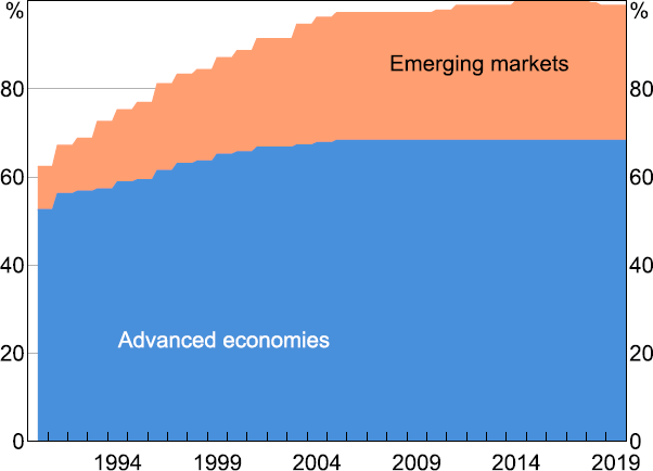
The foreign and global data were primarily collected from the St Louis Federal Reserve Economic Database (FRED) and the IMF International Financial Statistics (IFS) database. Variables that were missing from these sources were supplemented with data from Bloomberg, Reuters Refinitiv, CEIC and the Wind Financial Terminal. However, there are still some missing data, largely from series that only began to be published after 1990, with much of this being emerging market data (Figure 1). To estimate the factors using principal components, we fill in the missing data by applying Stock and Watson's (2002) expectations maximisation algorithm.
Data for the domestic Australian block were collected from the ABS or RBA statistical tables. The variables were gathered on a monthly or quarterly basis, as available, but we aggregate monthly variables to a quarterly frequency by taking their end-of-quarter levels to align the frequency of the available variables.[8] Due to data availability, and due to concerns that the volatility of the COVID-19 pandemic will significantly affect the results, we estimate the FAVAR using quarterly data from 1990 to the end of 2019.[9]
3.1.3 Description of the factors
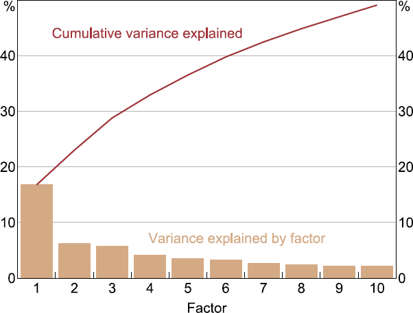
We estimate the factors using PCA on the panel of global data. Applying Bai and Ng's (2002) information criteria, we select three factors from the panel of foreign variables which cumulatively explain approximately 30 per cent of the variation in the data (Figure 2).[10] The PCA factors are orthogonal by construction. These factors cannot be interpreted as particular ‘structural’ shocks to the global economy, but rather capture the sum of the common global shocks that explain the most variation in the global panel. This approach illustrates the distinction between ‘global’ and ‘foreign’ shocks. To the extent that the factors only capture information that best explains common variation across the whole panel, we do not investigate how foreign shocks affecting only one country or one sector (i.e. that do not drive variation in broader global economic or financial conditions) affect the Australian economy.
In turn, we assume that these factors have the highest potential to explain the variation in Australian domestic variables.[11] While this prohibits us from assessing how any specific foreign shock affects the Australian economy, it allows us to assess how much of the variation in Australian data can be explained by common global shocks and through which channels they are transmitted to Australia.
In essence, our approach amounts to estimating how much the variation in the first several factors, which we assume adequately capture the relevant global shocks, explain variation in Australian economic and financial variables. We relax this assumption in Section 4.1.3 and explore whether other factors beyond the third factor drive a significant share of the variation in Australian data.
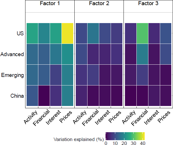
The first factor appears to explain substantial variation in categories of variables across the panel, especially for activity, interest rates and prices. The first factor has the strongest loading on US prices, explaining on average 41 per cent of variation for these variables (Figure 3 and Table B1). The third factor clearly explains more variation in financial variables than it does in other variables. The second factor is less clear, and it appears to loosely explain roughly equal variation in different types of variables, but seems to capture slightly more variation in US variables.
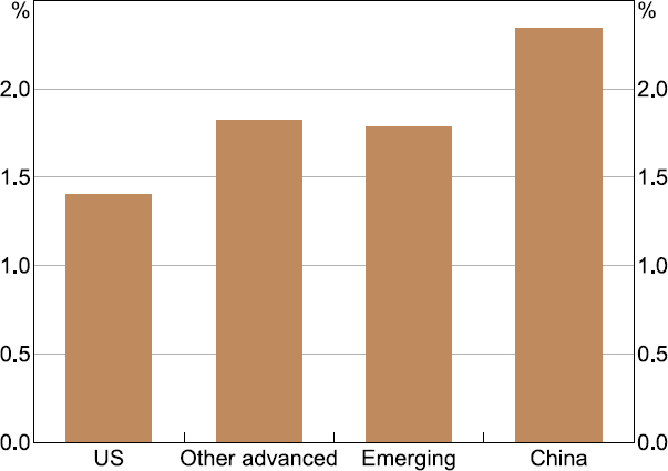
The first three factors together explain a particularly high proportion of variation in US variables, other advanced economy variables, and global variables, explaining 50 per cent, 29 per cent, and 35 per cent of the variation on average across the variables, respectively.[12] The factors explain noticeably less variation in variables for non-China emerging markets, explaining 21 per cent of the variation on average, and even less for China, where the factors explain 12 per cent of the variation on average. This may raise concerns that we are missing important shocks originating in China, which we address in Section 4.1.4.
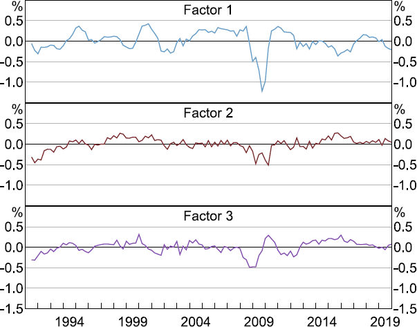
The first and third factor drop sharply during the GFC (Figure 4). This aligns with the interpretation of these factors as broadly relating to activity/prices and financial markets, respectively. The interpretation of the second factor is again less clear. While this may raise questions as to how to interpret these factors (a common issue in factor models), the specific interpretation of each factor is not particularly important as we do not attempt to use these factors to construct structural shocks for the purposes of the analysis in Section 4.
4. How Much Do Global Shocks Affect Australia?
We now use these estimated factors as the foreign block for our FAVAR. We first assess how much the global shocks captured by these factors matter for variables core to the mandate or toolkit of the RBA. Accordingly, for our domestic block, we use Australian quarterly headline CPI inflation, the (differenced) cash rate and unemployment rate, and (log differenced) nominal TWI and real GDP as a base specification.[13] To formalise the assumption that Australia is a small open economy, we impose that Australian variables do not affect the global factors contemporaneously or with a lag. Imposing these zero restrictions also helps to keep the model parsimonious.
4.1 Evidence from forecast error variance decompositions (FEVDs)
We explore the quantitative importance of global shocks for Australian variables through forecast error variance decompositions (FEVDs). These FEVDs show the sum of variation in our domestic variables that is explained by the global factors relative to the total forecast error variance of the domestic variables (the sum of variation driven by all global and domestic shocks). As is common when conducting inference on impulse response functions (though less common for FEVDs), we construct bootstrapped 68 per cent error bands around the point estimates of the joint contributions of global shocks to the forecast error variance of the domestic variables.[14]
4.1.1 Base specification
Global shocks as captured by our factors have heterogeneous effects on Australian domestic variables (Figure 5). In particular, global shocks appear to explain more variation in the cash rate and the nominal TWI than in headline CPI, real GDP, and, to some extent, the unemployment rate.[15] The finding that variation in the exchange rate and the policy rate is driven to a considerable extent by global shocks is in line with the literature on other small open economies and similar to earlier Australian studies (Jääskelä and Smith 2011; Manalo et al 2014), though the response of other economic variables, particularly GDP, is smaller (e.g. Vasishtha and Maier (2013) for Canada).[16] This observation accords with the notion that the Australian dollar buffers the economy from external shocks (RBA 2020).
These results also accord with the role of monetary policy in buffering the domestic economy from global shocks. Because the RBA targets domestic activity (unemployment) and inflation in line with its mandate, it moves the cash rate to buffer against external shocks that could knock domestic variables off the RBA's preferred path.[17] The nominal TWI appears to adjust to global shocks almost immediately, as seen by global shocks explaining an almost equal share of its variation on impact as at later horizons, in line with the efficient markets hypothesis (Cornell and Dietrich 1978). On the other hand, global shocks appear to feed through more slowly to the cash rate, suggesting these shocks may change the RBA's outlook with a lag, or that the RBA adjusts the cash rate gradually (Lowe and Ellis 1997). To the extent that global shocks could be affecting the RBA's outlook with a lag, this may reflect the fact that it takes time for the nature and size of global shocks to be understood, particularly if the RBA is predominantly responding to the global shock by waiting to see whether the shock affects domestic variables. Further investigating how precisely monetary policy responds to global shocks (and the extent to which policymakers wait to see a domestic effect) is a worthy matter for future research.
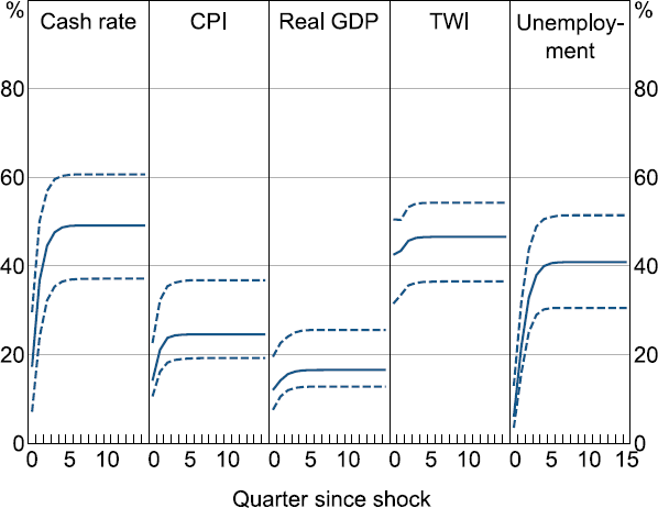
Note: Dashed lines show 68 per cent confidence interval.
A puzzling feature is that global shocks appear to explain significantly more variation in unemployment than in GDP, despite employment being an explicit mandate of the RBA rather than output. Moreover, in an Okun's Law framework, unemployment would be expected to move closely with GDP. One hypothesis is that quarterly real GDP is subject to considerably more measurement error than unemployment (Rees, Lancaster and Finlay 2014), or to temporary idiosyncratic shocks to non-labour-intensive sectors of the economy or sub-components (like non-monetary gold exports, which are highly volatile), and therefore moves less with global shocks than labour market indicators. Moreover, our results are also consistent with prior research that finds a relatively weak relationship between the output gap and the unemployment rate for Australia over our sample period (Lancaster and Tulip 2015).
Another possibility for the greater responsiveness of the labour market relative to output is that the exchange rate and cash rate buffer the Australian economy to remain relatively stable in aggregate, but the substitution of activity between sectors and regions still has noticeable effects on the labour market. This may be best seen through a narrative discussion of key episodes that drive material variation in our factors and the Australian variables. Australian quarterly real GDP growth, which is generally quite noisy, remained relatively stable through the 2001 US recession and the GFC that our first factor picks up as seen in Figure 4. On the other hand, unemployment did tick up in response to each of these episodes (Figure 6). During the GFC for example, the RBA noted that unemployment had risen despite the economy performing better than expected over the year. This coincided with a depreciation in the exchange rate which also brought on some compositional change: the labour markets in Western Australia and Queensland, relatively more mining-exposed and, therefore, export-exposed states, had been strong, while the labour market in New South Wales had deteriorated (RBA 2009a, 2009b).
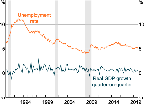
Notes: Seasonally adjusted. Shading indicates US recessions.
Sources: ABS; National Bureau of Economic Research.
Indeed, the mining sector has contributed an increasingly larger share of output, while its share of employment remains relatively low (more than 14 per cent of gross value added against around 2 per cent of employment in 2023). This itself suggests a potential reason that fluctuations in real GDP in recent decades have not been as tightly linked with fluctuations in unemployment as theory would suggest.
Our estimates for the effect of global shocks on GDP are also smaller than prior literature, especially the literature from the 2000s (e.g. Nimark 2007). While some of this may be driven by differences in methods used, it may also be driven by the way shocks originating in the United States are modelled and their changing relevance to Australia. In contrast to this paper, the prior literature almost exclusively studied spillovers from the United States to Australia. We address this issue next.
4.1.2 Comparison to a small-scale VAR
Part of the justification for applying the FAVAR approach in the context of assessing the contribution of global shocks is that it may better span the space of global shocks than a two-country model. We assess this claim by comparing the FEVDs for the base specification of the FAVAR with the results for a small-scale VAR with a foreign block made up solely of US variables.[18] We present the comparison between the FEVD results for the baseline FAVAR and the US foreign block VAR in Figure 7.
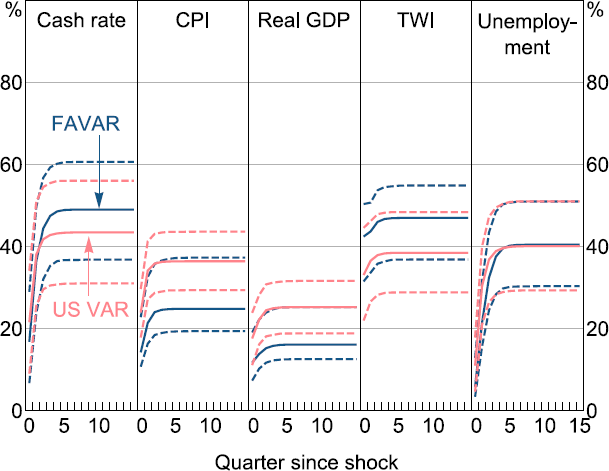
Note: Dashed lines show 68 per cent confidence intervals.
Compared to the small-scale VAR, the FAVAR captures shocks which explain more of the FEV in the cash rate and the TWI, a similar amount of variation in unemployment but less variation in CPI and real GDP, although the difference between the two models does not appear to be statistically significant for any variable. While it appears there are some shocks that the FAVAR is able to capture which a bilateral VAR is not, a US bilateral VAR captures a substantial proportion of the relevant shocks, likely due to the US economy's central importance in the global economy. This does not necessarily mean that the US economy is more important to Australia than the global economy, but it does suggest that variation in US economic and financial variables over 1990–2019 were effectively a ‘sufficient statistic’ for capturing global economic shocks, and indeed possibly better capture global information relevant to Australia's inflation and GDP growth.
4.1.3 Exploring the role of additional factors
So far, we have estimated the baseline FAVAR using the factors that best explain variation in our panel of global data (this being the purpose of PCA estimation). However, these are not necessarily the same factors that best explain variation in Australian data. We therefore test whether there are other principal components which do not explain variation in the global panel as well, but explain more of the variation in Australian data. To do this we experiment with adding a fourth factor to the baseline FAVAR. We start with the fourth principal component, and then replace that factor one by one with each of the 116 other principal components we calculate, each time assessing the average FEV explained across the Australian variables by all foreign factors when including this particular principal component.
Adding any one of these factors does not explain substantially more variation in the Australian variables than the baseline specification (Figure 8). Regardless, we investigate whether there is some systematic similarity between the excluded factors that explain more variation in Australian variables.
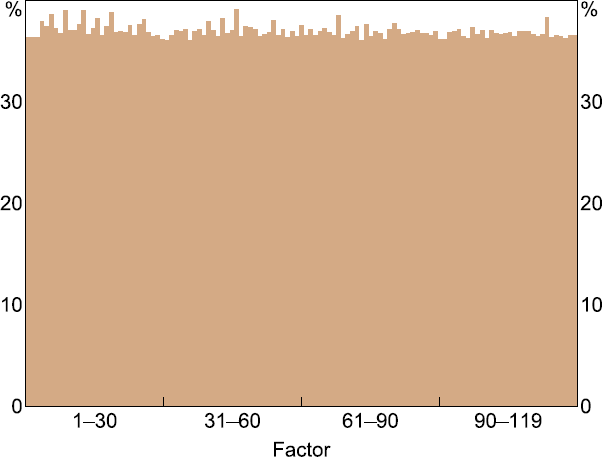
For this, we rank the models shown in Figure 8 and select the five that explain the highest proportion of FEV in the Australian data. These five factors on average explain greater variation in Chinese variables than in variables from other countries (Figure 9). This is unlike the first three principal components we use in the baseline specification, which explain very little variation in Chinese variables (Figure 3).
This suggests that factors that are idiosyncratic to the Chinese economy are more relevant for explaining variation in the Australian economy than explaining variation across the global panel more broadly. This aligns with the particular importance of the Chinese economy to Australia, which comes largely from trade (Guttmann et al 2019). Overall, however, the variation explained in Chinese variables by the alternative fourth factors are relatively low, and the FEV explained by global factors when including the alternative ‘China’ factors is not significantly different from the baseline FEVD.
4.1.4 Are we missing important shocks originating in China?
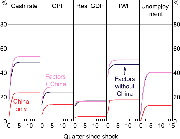
To test if the low loadings on Chinese variables are leading to lower FEV explained in the Australian data than if we allowed these Chinese variables to directly affect Australian variables, we conduct three further experiments. First, we test a model with the original three factors when estimated on a global panel without any Chinese data. Second, we test a model with the global factors excluding China but explicitly adding four Chinese variables to the foreign block: GDP, industrial production, 10-year government bond yield and CPI. As there may be concerns about measurement error in Chinese GDP data affecting the results, we use the Chinese GDP measure from Barcelona et al (2022), which is generated from a dynamic factor model on a variety of Chinese activity data. Third, we test a bilateral VAR with only the four Chinese variables mentioned alone as the foreign block. We present the FEVDs for the three experiments in Figure 10.
At face value, the results suggest that shocks reflected in Chinese data do not explain material variation in key Australian economic variables. There is little difference between the FEV explained in the Australian data by the model using the factors without China alone and the model with the same factors without China but also including Chinese variables explicitly. The model with the factors without China and additional Chinese variables also explains only marginally more of the variation in the Australian data than the baseline three factors, despite having a considerably richer foreign block. Consistent with that, using the Chinese variables alone explains significantly less of the FEV in Australian variables.
This could suggest that shocks originating in other advanced economies are more important to Australia's economic outcomes than shocks originating from China. On the other hand, Chinese shocks may be just as important for Australia, but shocks originating from China are captured in large part by other global data, while Chinese data are not capturing shocks from other countries. This could be the case for instance if Chinese government policy is explicitly insulating the Chinese economy from global shocks, whereas shocks from the Chinese economy are having observable effects on global data. A third hypothesis is that Chinese shocks are important in explaining the long-run levels of Australian variables, but do not explain substantial short-run variation. Without explicitly identifying the particular shocks, we cannot distinguish between the three hypotheses.
This result may be somewhat surprising, given that China's demand for Australia's mining exports has been a very significant factor in supporting Australian exports, and particularly contributed to the stability of the Australian economy during the GFC after Chinese authorities implemented a major stimulus package at the end of 2008. To some degree, the result reflects the particular time period of our sample and our modelling approach. For one, in the early part of the sample period China was less significant for the global economy and less open than in recent years, particularly prior to entering the World Trade Organization in the early 2000s. By contrast, in the later part of the sample China would be expected to have a larger effect on the Australian economy. Therefore over the whole sample, China's impact may appear more muted.
Secondly, the characteristics of the Australian mining industry may mute the measured impact of cyclical shocks originating in China in our model. Over our sample, Australia has been most exposed to slower-moving structural change in China, in particular through increased demand for Australian commodities. However, mines are long-lived and have long lead times on capital expenditure, which are planned years in advanced. These characteristics mean that the rise in Chinese demand for Australian commodities is highly visible in the Australian macroeconomy over the medium term, such as in the increase in the gross value added of the mining sector. However, the effects of Chinese shocks on the Australian economy are difficult to identify using shorter-run variation in quarter-to-quarter growth, which is what the FAVAR model relies on.
5. How Do Global Shocks Spill Over to Australia?
Traditional models would suggest that global shocks primarily spill over through adjustments in exchange rates and trade, as discussed in Section 1. However, more recent literature has emphasised the importance of global banks as a transmission channel for global shocks (Miranda-Agrippino and Rey 2020). We therefore test the importance of this channel for Australia.
5.1 A domestic block with financial variables
To assess the role of the Australian banking system in transmitting global shocks, we first augment the baseline domestic block in the VAR with Australian financial variables. We add one domestic financial variable to the baseline domestic block and re-estimate the contribution to the FEV by global shocks, replacing the domestic financial variable each time. In particular, we add log differences in: an index of Australian housing prices, the ASX all ordinaries index, value of deposits at banks in Australia, outstanding loans by banks in Australia, and differences in the spread between business lending rates and the bank bill swap rate (a measure of financial stress, see Beckers (2020)).
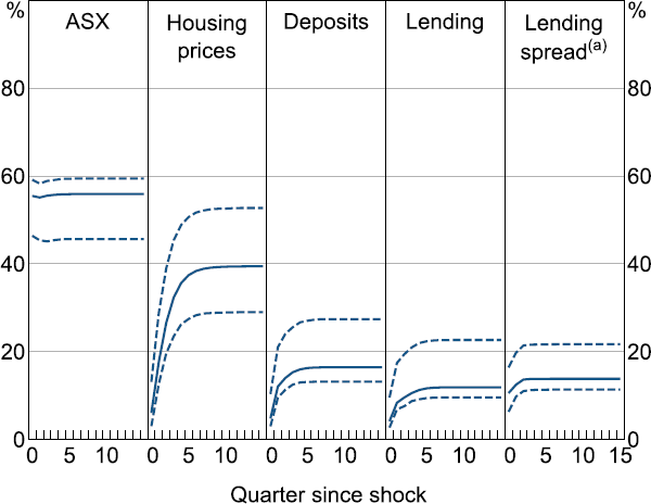
Global shocks explain a large share of the FEV of stock prices, as well as housing prices (Figure 11). In line with the efficient markets hypothesis, stock prices appear to adjust to global shocks almost immediately, as seen by global shocks explaining an almost equal share of their variation on impact as at later horizons. On the other hand, global shocks explain an increasingly greater proportion of FEV in housing prices over time, which could suggest these prices are not directly affected by the global shocks, but that this effect is instead intermediated by the response of other domestic variables such as the cash rate. Alternatively, this would be consistent with the housing market being slow moving and repricing less efficiently in response to shocks than equity prices. The global shocks explain very little of the FEV in Australian deposits, lending and lending spreads.[19]
Since global shocks appear to explain substantial variation in some other domestic variables (like unemployment and housing prices) without explaining substantial variation in banking variables, this suggests that global shocks are spilling over not via bank lending but by one of the other channels. For example, the substantial proportion of the FEV in the TWI explained by the global shocks would align with an exchange rate channel, while the results for stock prices and housing prices would be consistent with an asset price channel. While we are unable to say which of the two channels is more likely to explain spillovers to Australia, a lack of reaction by banking variables to global shocks suggests that the banking channel is not a main channel for spillovers of global shocks to Australia. In contrast, global shocks explain considerably more variation in the exchange rate and somewhat more variation in certain trade variables, suggesting that traditional models of spillovers may be a better description for the Australian economy (see Appendix C).
Notes:
Dashed lines show 68 per cent confidence interval.
(a) Spread between average lending rates and the three-month bank bill swap rate.
5.2 Impulse response functions to ‘shocks’ in global factors
To further investigate how financial variables respond to global shocks, we compute impulse response functions (IRFs) for ‘shocks’ in the global factors. As we are not imposing any structural identification within the foreign block, these are not interpretable as the response of Australian variables to any particular structural shock. The small open economy assumption of Australian shocks not having an effect on the global factors is sufficient to identify that a shock is global, but not precisely what kind of shock it is. For instance, shocking the third factor, which appears to reflect variation in financial variables primarily, is not interpretable as a financial shock, as without an identification approach it may be picking up any underlying combination of global shocks, such as a combination of a simultaneous shock to aggregate demand and financial risk.
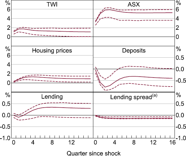
However, if a given Australian variable does not respond to a shock to a given factor, this at least suggests that it is unlikely that the variable is an important channel of transmission for the global shocks. In other words, we would expect some response of a variable if it were a significant channel of spillovers in Australia, unless the underlying shocks are a linear combination of shocks that happen to perfectly cancel out the effect on the Australian variable. We present the cumulated IRFs for several financial variables to a one standard deviation shock of the third factor that loads most strongly on financial variables in Figure 12.[20] Several features of the IRFs to a shock in the third factor are consistent with the analysis of the FEVDs.
Notes:
Dashed lines show 68 per cent confidence interval.
(a) Spread between average lending rates and three-month bank bill swap rate.
The TWI initially appreciates by around 1 per cent in response to the shock and remains at that level over the horizon. Asset prices respond positively to the shock, with the level of the ASX all ordinaries index increasing 5 per cent and housing prices increasing 1 per cent. The banking variables – lending, deposits and lending spread – all show a close to zero or statistically insignificant response by the end of the horizon. This corroborates the FEVD evidence for banks not acting as a major channel for the shock to spill over to other domestic variables. This is in contrast to the findings of Miranda-Agrippino and Rey (2020) that deposits, lending and financing costs are the dimensions of the banking channel for the transmission of global shocks. We report the responses of the baseline block of variables in Appendix C (Figure C2).
6 Discussion
Our results highlight that global shocks can have significant effects on the Australian economy. However, the shocks appear to spill over to Australia via some channel other than the banking channel, which raises the question: what is different about Australia's banking sector?
6.1 Why is the Australian banking response to global shocks relatively small?
There are several reasons why the Australian banking system may be more insulated from global shocks than the banking system of other countries, which we will discuss in turn:
- Australian banks trade securities on their own accounts less than global banks and are instead engaged more in domestic home lending. Australian banks are also more hedged than major global banks, with most foreign (and domestic) currency debt hedged back to the Australian bank bill swap rate.
- The Australian banking system is more concentrated than the banking systems of some other advanced economies, with particularly little participation by foreign banks. Australian banks are more profitable than their global counterparts, especially in the home-lending segment. They also tend to be less leveraged than major global banks.
6.1.1 A banking system focused on domestic home lending, with well-hedged offshore funding
Miranda-Agrippino and Rey (2020) explain the role of global banks as a spillover channel for global shocks, using a model where global banks adjust their holdings of a portfolio of dollar-denominated risky securities in response to changes in the US risk-free rate (the rate at which they fund themselves). This description may be appropriate for global banks operating in regions such as the euro area, however, Australian banks appear to be less exposed to global shocks both on the asset and liability side of their books.
On the asset side, Australian banks trade securities on their own accounts considerably less than global banks. Amongst the 50 largest global banks by total assets (which includes all of Australia's Big 4 banks), the Australian banks had a lower-than-average amount of marketable securities as a proportion of their assets, and lower-than-average trading profits as a proportion of total net income in 2022 (Figure 13).[21] The importance of traditional lending for the Australian banks is reflected in the higher average total loans to total assets for Australian banks than other global banks.
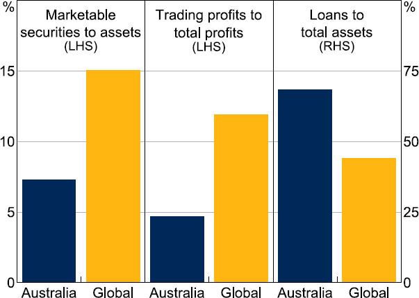
Note: Top 50 global banks by market capitalisation, excluding Chinese banks.
Sources: Authors' calculations; Bloomberg.
On the liability side, as Atkin and Harris (2023) and Johnson (2022) point out, Australian offshore funding tends to be exchange rate-hedged. Banks issuing bonds offshore are the main source of foreign currency exposure for the sector, but around 90 per cent of these liabilities are hedged using derivatives. As illustrated in Figure 14, from Atkin and Harris (2023), after hedging, the Australian banking sector had a net foreign currency asset position in 2022, and no significant currency mismatches, both of which reduce the risk from an exchange rate depreciation. While foreign banks' exchange rate hedge ratios are not directly observable, the lower absolute exchange rate effect on cash flow as a proportion of net income for Australian banks' compared to major foreign banks in 2021 suggests that Australian banks may hedge their exchange rate risk more fully (Figure 15).[22] Australian banks also tend to account for interest rate risk by hedging exposures back to the domestic bank bill swap rate (Fitzpatrick et al 2022). Interest rate hedging by banks in the United States and euro area on the other hand tends to be less prevalent (Beganau, Piazzesi and Schneider 2015; Hoffmann et al 2019).
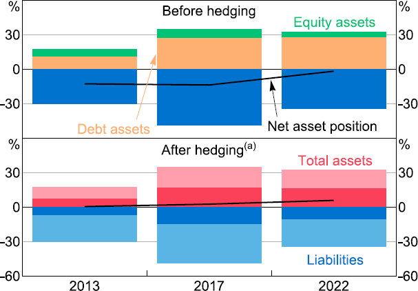
Note: (a) Lighter shaded bars indicate hedged component.
Source: Atkin and Harris (2023).
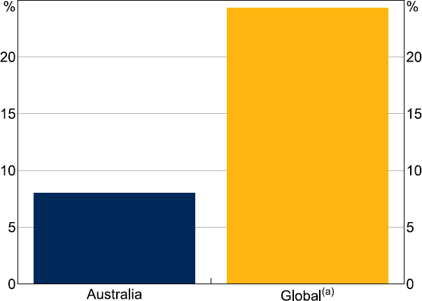
Note: (a) Top 50 global banks by market capitalisation, excluding Chinese banks.
Sources: Authors' calculations; Bloomberg.
6.1.2 Concentration, profitability and leverage
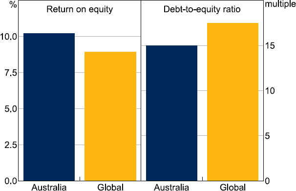
The Australian banking system is relatively highly concentrated (Figure 16), and Australia's major banks are relatively profitable compared to global banks (Figure 17) (Bullock 2017).
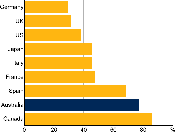
Note: Share of assets for euro area countries, share of loans for all other countries.
Sources: APRA; Authors' calculations; Bloomberg.
Both of these features may have reduced Australia's banking exposure to global shocks in the past. First, this is because foreign banks, which may be more likely to transmit shocks from their home markets than domestic banks, have only a minor presence in the Australian banking sector. By comparison, Australian banks' foreign exposures, other than the hedged liabilities discussed above, largely come in the form of banking activities in the New Zealand market (Bellrose and Norman 2019). Second, Australian banks' high profitability, all else equal, makes it easier for them to generate capital through retained earnings, and they are therefore less likely to be forced to deleverage as a result of coming up against the mandated minimums for their capital ratios, should they be hit by global shocks. Australian banks also tend to be less leveraged in the first place, which goes towards the same argument (Figure 17).
However, these features do not necessarily suggest that spillovers through the Australian banking sector will always be muted. As Bullock (2017) points out, banking sector concentration could also lead to a ‘too big to fail’ dynamic. For example, if a major bank was highly exposed to a particular global shock, then the concentration of the banking sector would amplify that shock rather than mute its effects. That is, in combination the concentration of the Australian banking sector and these other features may insulate the Australian banking system from global shocks, but considered alone, concentration could theoretically lead to greater spillovers of global shocks.
Note: Top 50 global banks by market capitalisation, excluding Chinese banks.
Sources: Authors' calculations; Bloomberg.
6.2 Implications
This work suggests that global economic and financial developments, particularly in the United States and for other advanced economies, can have substantial effects on the Australian economy. However, this analysis also suggests that for Australia, channels other than the international banking channel, such as the exchange rate, trade, and asset price channels are likely more important when assessing spillovers of global shocks. That being said, the features of the Australian banking system which have made this channel less prevalent over our sample are also endogenous to Australian financial regulation and global financial trends. Any changes in the institutional structure of the Australian banking sector may therefore change how global shocks affect Australia.
This work also suggests that future academic research should more closely examine the extent to which the importance of the international banking channel of global shocks is driven by the particular structure of countries' banking systems. Prior papers such as Buch et al (2019) have provided important evidence for the relevance of this channel. In that paper, the authors identify the effects of foreign policy on countries' bank balance sheets from heterogeneity in banks' foreign funding exposures. However, the countries with sufficient bank heterogeneity to be exploited usefully with the chosen econometric approach may be precisely the countries where spillovers through the international banking channel are larger, weakening the external validity of the results. That is, a concentrated banking system where all banks have minimal unhedged foreign exposures may be both less susceptible to investigation using this method and less likely to experience spillovers via the international banking channel. Further research could test the evidence for the international banking channel produced by other countries with banking systems more like Australia's.
7 Conclusion
We examine the extent to which global shocks affect the Australian financial and economic variables using a FAVAR model. We find that global shocks explain substantial variation in variables that are thought to buffer the economy from global shocks (the exchange rate and the cash rate), but less variation in other economic variables (especially real GDP). Recent literature on global spillovers has particularly focused on the international banking channel as a carrier of global shocks. However, we find that the response of Australian banking sector variables to global shocks are inconsistent with this channel being the primary driver of spillovers to Australia. We suggest several features of the Australian banking sector that may drive this result, particularly around funding and lending behaviour, and bank risk management.
Future research could also more closely examine how the characteristics of countries' banking systems affect estimates of the importance of the international banking channel as a carrier of global shocks. Another avenue for further research could be to examine the extent to which the cash rate acts as a buffer against global shocks directly (i.e. directly viewing and responding to global variables) or indirectly (in response to domestic economic variables moving as a consequence of the global shock). If the cash rate response tends to be indirect, as the lagged response in the cash rate may suggest, then a useful line of research could be to determine which global variables fluctuations most accurately signal an imminent domestic effect.
Appendix A: Data
| Country/Region | Variable | Source | Transformation | Available from |
|---|---|---|---|---|
| Asia | Corporate bond yield index spread | Bloomberg | First difference | Sep 2001 |
| Canada | 10-year government bond yield | St. Louis FRED | First difference | Jan 1990 |
| Canada | 90-day interbank rate | St. Louis FRED | First difference | Jan 1990 |
| Canada | CPI | IMF IFS | Log difference | Jan 1990 |
| Canada | Exchange rate to US dollar | St. Louis FRED | Log difference | Jan 1990 |
| Canada | Final consumption index | IMF IFS | Log difference | Mar 1990 |
| Canada | GDP deflator | IMF IFS | Log difference | Mar 1990 |
| Canada | Industrial production index | IMF IFS | Log difference | Jan 1997 |
| Canada | Investment | IMF IFS | Log difference | Mar 1990 |
| Canada | Net exports | IMF IFS | Log difference | Mar 1990 |
| Canada | Policy rate | Reuters Refinitiv | First difference | Jan 1990 |
| Canada | Producer price index | Reuters Refinitiv | Log difference | Jan 1990 |
| Canada | Real GDP | IMF IFS | Log difference | Mar 1990 |
| Canada | Total share price index | St. Louis FRED | Log difference | Jan 1990 |
| Canada | Unemployment rate | IMF IFS | First difference | Jan 1990 |
| China | 10-year government bond yield | Bloomberg | First difference | Jun 2005 |
| China | 90-day interbank rate | Bloomberg | First difference | Sep 2014 |
| China | CPI | IMF IFS | Log difference | Jan 1990 |
| China | Exchange rate to US dollar | St. Louis FRED | Log difference | Jan 1990 |
| China | Industrial production index | CEIC | Log difference | Jan 1994 |
| China | Producer price index | Reuters Refinitiv | Log difference | Jan 1993 |
| China | Reserve requirement ratio | CEIC | First difference | Jan 1994 |
| China | Total stock price index (Shanghai Composite) | Bloomberg | Log difference | Dec 1990 |
| China | Unemployment rate | Reuters Refinitiv | First difference | Mar 2004 |
| Emerging markets | JP Morgan Emerging Market volatility index | Bloomberg | First difference | Mar 2000 |
| Euro area | Corporate bond yield index spread | Bloomberg | First difference | Jun 1998 |
| Euro area | ECU/euro to US dollar | Bloomberg | Log difference | Jan 1990 |
| Euro area | Eurostoxx VIX | Bloomberg | Log difference | Mar 1999 |
| France | 10-year government bond yield | St. Louis FRED | First difference | Jan 1990 |
| France | 90-day interbank rate | St. Louis FRED | First difference | Jan 1990 |
| France | CPI | IMF IFS | Log difference | Jan 1990 |
| France | Final consumption index | IMF IFS | Log difference | Mar 1990 |
| France | GDP deflator | IMF IFS | Log difference | Mar 1990 |
| France | Import price index | IMF IFS | Log difference | Jan 1999 |
| France | Industrial production index | IMF IFS | Log difference | Jan 1990 |
| France | Net exports | IMF IFS | Log difference | Mar 1990 |
| France | Producer price index | Reuters Refinitiv | Log difference | Jan 1995 |
| France | Real GDP | IMF IFS | Log difference | Mar 1990 |
| France | Total share price index | St. Louis FRED | Log difference | Jan 1990 |
| France | Unemployment rate | IMF IFS | First difference | Jan 2003 |
| Germany | 10-year government bond yield | St. Louis FRED | First difference | Jan 1990 |
| Germany | 90-day interbank rate | St. Louis FRED | First difference | Jan 1990 |
| Germany | CPI | IMF IFS | Log difference | Jan 1990 |
| Germany | Final consumption index | IMF IFS | Log difference | Mar 1991 |
| Germany | GDP deflator | IMF IFS | Log difference | Mar 1991 |
| Germany | Import price index | IMF IFS | Log difference | Jan 1990 |
| Germany | Industrial production index | IMF IFS | Log difference | Jan 1990 |
| Germany | Investment | Reuters Refinitiv | Log difference | Mar 1991 |
| Germany | Net exports | IMF IFS | Log difference | Mar 1991 |
| Germany | Producer price index | IMF IFS | Log difference | Jan 1990 |
| Germany | Real GDP | IMF IFS | Log difference | Mar 1991 |
| Germany | Total share price index | St. Louis FRED | Log difference | Jan 1990 |
| Germany | Unemployment rate | Reuters Refinitiv | First difference | Mar 2004 |
| Global | Base metals price index | RBA | Log difference | Jan 1990 |
| Global | Brent oil price | St. Louis FRED | Log difference | Jan 1990 |
| Global | Bulks price index | RBA | Log difference | Jan 1990 |
| Global | Global exchange rate volatility index | Bloomberg | First difference | Jun 1992 |
| Global | Rural commodities price index | RBA | Log difference | Jan 1990 |
| Global | WTI oil | St. Louis FRED | Log difference | Jan 1990 |
| India | 10-year government bond yield | St. Louis FRED | First difference | Dec 2011 |
| India | 90-day interbank rate | St. Louis FRED | First difference | Dec 2011 |
| India | CPI | IMF IFS | Log difference | Jan 1990 |
| India | Exchange rate to US dollar | St. Louis FRED | Log difference | Jan 1990 |
| India | Final consumption index | IMF IFS | Log difference | Jun 1996 |
| India | GDP deflator | IMF IFS | Log difference | Jun 1996 |
| India | Industrial production index | IMF IFS | Log difference | Jan 1990 |
| India | Net exports | IMF IFS | Log difference | Jun 1996 |
| India | Policy rate | IMF IFS | First difference | Jun 2000 |
| India | Producer price index | IMF IFS | Log difference | Apr 2004 |
| India | Real GDP | IMF IFS | Log difference | Jun 1996 |
| India | Total share price index | St. Louis FRED | Log difference | Jan 1990 |
| Italy | 10-year government bond yield | St. Louis FRED | First difference | Jun 1993 |
| Italy | 90-day interbank rate | St. Louis FRED | First difference | Jan 1990 |
| Italy | CPI | IMF IFS | Log difference | Jan 1990 |
| Italy | Final consumption index | IMF IFS | Log difference | Mar 1996 |
| Italy | GDP deflator | IMF IFS | Log difference | Mar 1996 |
| Italy | Import price index | IMF IFS | Log difference | Jan 2005 |
| Italy | Industrial production index | IMF IFS | Log difference | Jan 1990 |
| Italy | Net exports | IMF IFS | Log difference | Mar 1996 |
| Italy | Producer price index | IMF IFS | Log difference | Jan 1991 |
| Italy | Real GDP | IMF IFS | Log difference | Mar 1996 |
| Italy | Total share price index | St. Louis FRED | Log difference | Jan 1990 |
| Italy | Unemployment rate | IMF IFS | First difference | Jan 1990 |
| Japan | 10-year government bond yield | St. Louis FRED | First difference | Jan 1990 |
| Japan | 90-day interbank rate | St. Louis FRED | First difference | Jan 1990 |
| Japan | CPI | IMF IFS | Log difference | Jan 1990 |
| Japan | Exchange rate to US dollar | St. Louis FRED | Log difference | Jan 1990 |
| Japan | Final consumption index | IMF IFS | Log difference | Mar 1990 |
| Japan | GDP deflator | IMF IFS | Log difference | Mar 1994 |
| Japan | Import price index | IMF IFS | Log difference | Jan 1990 |
| Japan | Industrial production index | IMF IFS | Log difference | Jan 1990 |
| Japan | Investment | IMF IFS | Log difference | Mar 1994 |
| Japan | Net exports | IMF IFS | Log difference | Mar 1990 |
| Japan | Policy rate | IMF IFS | First difference | Mar 1990 |
| Japan | Producer price index | IMF IFS | Log difference | Jan 1990 |
| Japan | Real GDP | IMF IFS | Log difference | Mar 1990 |
| Japan | Total share price index | St. Louis FRED | Log difference | Jan 1990 |
| Japan | Unemployment rate | IMF IFS | First difference | Jan 1990 |
| Latin America | Corporate bond yield index spread | Bloomberg | First difference | Sep 2001 |
| Mexico | 10-year government bond yield | St. Louis FRED | First difference | Jul 2001 |
| Mexico | 90-day interbank rate | St. Louis FRED | First difference | Jan 1997 |
| Mexico | CPI | IMF IFS | Log difference | Jan 1990 |
| Mexico | Exchange rate to US dollar | St. Louis FRED | Log difference | Nov 1993 |
| Mexico | Final consumption index | IMF IFS | Log difference | Mar 1993 |
| Mexico | GDP deflator | IMF IFS | Log difference | Mar 1993 |
| Mexico | Import price index | IMF IFS | Log difference | Feb 2014 |
| Mexico | Industrial production index | IMF IFS | Log difference | Jan 1990 |
| Mexico | Net exports | IMF IFS | Log difference | Mar 1993 |
| Mexico | Policy rate | IMF IFS | First difference | Dec 2001 |
| Mexico | Producer price index | IMF IFS | Log difference | Dec 2003 |
| Mexico | Real GDP | IMF IFS | Log difference | Mar 1993 |
| Mexico | Total share price index | St. Louis FRED | Log difference | Jan 1990 |
| Mexico | Unemployment rate | IMF IFS | First difference | Jun 1995 |
| New Zealand | 10-year government bond yield | St. Louis FRED | First difference | Jan 1990 |
| New Zealand | 90-day interbank rate | St. Louis FRED | First difference | Jan 1990 |
| New Zealand | CPI | IMF IFS | Log difference | Mar 1990 |
| New Zealand | Exchange rate to US dollar | St. Louis FRED | Log difference | Jan 1990 |
| New Zealand | Final consumption index | IMF IFS | Log difference | Mar 1990 |
| New Zealand | GDP deflator | IMF IFS | Log difference | Mar 1990 |
| New Zealand | Import price index | IMF IFS | Log difference | Mar 1990 |
| New Zealand | Industrial production index | St. Louis FRED | Log difference | Jan 1990 |
| New Zealand | Investment | IMF IFS | Log difference | Mar 1990 |
| New Zealand | Net exports | IMF IFS | Log difference | Mar 1990 |
| New Zealand | Policy rate | IMF IFS | First difference | Mar 1999 |
| New Zealand | Producer price index | IMF IFS | Log difference | Mar 1990 |
| New Zealand | Real GDP | IMF IFS | Log difference | Mar 1990 |
| New Zealand | Total share price index | St. Louis FRED | Log difference | Jan 1990 |
| New Zealand | Unemployment rate | IMF IFS | First difference | Mar 1990 |
| Russia | 10-year government bond yield | St. Louis FRED | First difference | Jan 1999 |
| Russia | CPI | IMF IFS | Log difference | Jan 1992 |
| Russia | Exchange rate to US dollar | St. Louis FRED | Log difference | Jun 1992 |
| Russia | Final consumption index | IMF IFS | Log difference | Mar 2003 |
| Russia | GDP deflator | IMF IFS | Log difference | Mar 2003 |
| Russia | Industrial production index | IMF IFS | Log difference | Jan 1995 |
| Russia | Net exports | IMF IFS | Log difference | Mar 2003 |
| Russia | Policy rate | IMF IFS | First difference | Dec 2001 |
| Russia | Producer price index | Reuters Refinitiv | Log difference | Jan 1991 |
| Russia | Real GDP | IMF IFS | Log difference | Mar 2003 |
| Russia | Total share price index | St. Louis FRED | Log difference | Sep 1997 |
| Russia | Unemployment rate | IMF IFS | First difference | Jan 2010 |
| South Korea | 10-year government bond yield | St. Louis FRED | First difference | Oct 2000 |
| South Korea | 90-day interbank rate | Bloomberg | First difference | Sep 1998 |
| South Korea | CPI | IMF IFS | Log difference | Jan 1990 |
| South Korea | Exchange rate to US dollar | St. Louis FRED | Log difference | Jan 1990 |
| South Korea | Final consumption index | IMF IFS | Log difference | Mar 1990 |
| South Korea | GDP deflator | IMF IFS | Log difference | Mar 1990 |
| South Korea | Import price index | IMF IFS | Log difference | Jan 1990 |
| South Korea | Industrial production index | IMF IFS | Log difference | Jan 1990 |
| South Korea | Investment | IMF IFS | Log difference | Mar 1990 |
| South Korea | Net exports | IMF IFS | Log difference | Mar 1990 |
| South Korea | Policy rate | IMF IFS | First difference | May 1999 |
| South Korea | Producer price index | IMF IFS | Log difference | Jan 1990 |
| South Korea | Real GDP | IMF IFS | Log difference | Mar 1990 |
| South Korea | Total share price index | St. Louis FRED | Log difference | Jan 1990 |
| South Korea | Unemployment rate | IMF IFS | First difference | Jan 1990 |
| UK | 10-year government bond yield | St. Louis FRED | First difference | Jan 1990 |
| UK | 90-day interbank rate | St. Louis FRED | First difference | Jan 1990 |
| UK | CPI | IMF IFS | Log difference | Jan 1990 |
| UK | Exchange rate to US dollar | St. Louis FRED | Log difference | Jan 1990 |
| UK | Final consumption index | IMF IFS | Log difference | Mar 1990 |
| UK | GDP deflator | IMF IFS | Log difference | Mar 1990 |
| UK | Import price index | IMF IFS | Log difference | Mar 1997 |
| UK | Industrial production index | IMF IFS | Log difference | Jan 1990 |
| UK | Investment | IMF IFS | Log difference | Mar 1990 |
| UK | Net exports | IMF IFS | Log difference | Mar 1990 |
| UK | Policy rate | IMF IFS | First difference | Jan 1990 |
| UK | Producer price index | IMF IFS | Log difference | Jan 1990 |
| UK | Real GDP | IMF IFS | Log difference | Mar 1990 |
| UK | Total share price index | St. Louis FRED | Log difference | Jan 1990 |
| UK | Unemployment rate | IMF IFS | First difference | Jan 1990 |
| US | 10-year government bond yield | St. Louis FRED | First difference | Jan 1990 |
| US | 90-day interbank rate | St. Louis FRED | First difference | Jan 1990 |
| US | Corporate Baa 10-year spread | Bloomberg | First difference | Mar 1990 |
| US | CPI | IMF IFS | Log difference | Jan 1990 |
| US | Final consumption index | IMF IFS | Log difference | Mar 1990 |
| US | GDP deflator | IMF IFS | Log difference | Mar 1990 |
| US | ICE corporate bond high yield index spread | St. Louis FRED | First difference | Mar 1994 |
| US | Import price index | IMF IFS | Log difference | Mar 1997 |
| US | Industrial production index | IMF IFS | Log difference | Jan 1990 |
| US | Investment | IMF IFS | Log difference | Mar 1990 |
| US | Net exports | IMF IFS | Log difference | Mar 1990 |
| US | Policy rate | IMF IFS | First difference | Jan 1990 |
| US | Producer price index | IMF IFS | Log difference | Jan 1990 |
| US | Real GDP | IMF IFS | Log difference | Mar 1990 |
| US | Total share price index | St. Louis FRED | Log difference | Jan 1990 |
| US | Unemployment rate | IMF IFS | First difference | Jan 1990 |
| US | VIX | St. Louis FRED | First difference | Mar 1990 |
Appendix B: Factor Loadings
| Factor | Category | Region type | ||||
|---|---|---|---|---|---|---|
| US | Advanced | Emerging | China | Global | ||
| Factor 1 | Activity | 24.9 | 14.9 | 14.5 | 13.3 | |
| Factor 1 | Financial | 18.9 | 12.7 | 9.6 | 0.2 | 16.0 |
| Factor 1 | Interest | 24.2 | 16.6 | 6.9 | 5.1 | |
| Factor 1 | Prices | 40.7 | 20.7 | 18.0 | 18.1 | |
| Factor 1 | Commodities | 30.4 | ||||
| Factor 2 | Activity | 9.5 | 9.6 | 5.9 | 1.3 | |
| Factor 2 | Financial | 14.8 | 3.9 | 10.5 | 1.0 | 1.1 |
| Factor 2 | Interest | 9.3 | 4.0 | 1.6 | 1.8 | |
| Factor 2 | Prices | 8.1 | 6.5 | 2.5 | 0.7 | |
| Factor 2 | Commodities | 5.6 | ||||
| Factor 3 | Activity | 5.4 | 1.6 | 2.8 | 3.5 | |
| Factor 3 | Financial | 32.1 | 18.1 | 11.9 | 0.5 | 2.0 |
| Factor 3 | Interest | 5.3 | 2.0 | 1.7 | 2.6 | |
| Factor 3 | Prices | 10.2 | 9.1 | 1.1 | 1.3 | |
| Factor 3 | Commodities | 5.8 | ||||
|
Note: Blank cells represent no variables captured by the country/category pairs. |
||||||
Appendix C: Supplementary VAR Results
C.1 Trade FEVDs
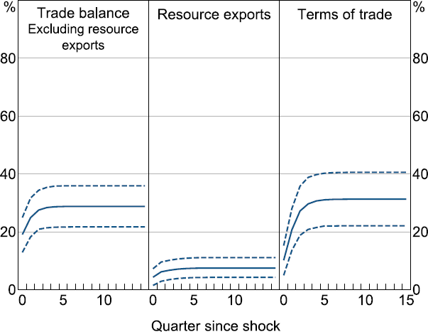
The global shocks explain close to 30 per cent of the FEV for Australia's terms of trade and for the goods and services trade balance when subtracting resource exports. The global shocks explain very little of the variation in resource exports. Although long-run trends in resource exports clearly depend on foreign demand, Australian producers of some commodities (especially iron ore) are generally low-cost producers compared to global competitors, such that they tend to produce to their maximum capacity regardless of shifts in demand (RBA 2015). Therefore short-run variation in volumes is likely to be driven more by supply shocks than demand shocks. Prices on the other hand appear more responsive to demand.
Note: Dashed lines show 68 per cent confidence interval.
C.2 Impulse response functions
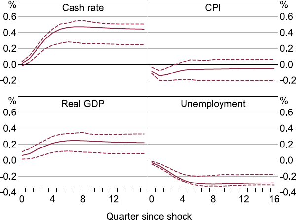
IRFs for a shock to the third factor
Note: Dashed lines show 68 per cent confidence interval.
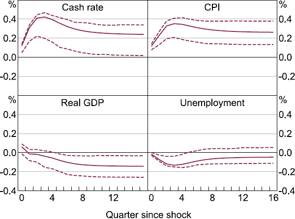
IRFs for a shock to the first factor
Note: Dashed lines show 68 per cent confidence interval.
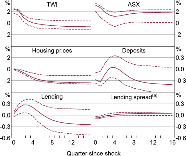
Notes:
Dashed lines show 68 per cent confidence interval.
(a) Spread between average lending rates and three-month bank bill swap rate.
IRFs for a shock to the second factor
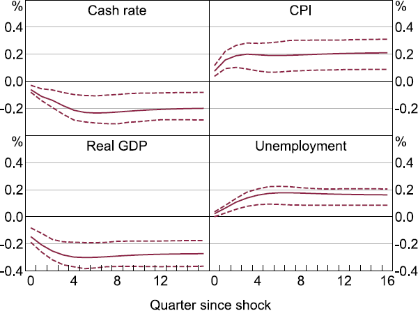
Note: Dashed lines show 68 per cent confidence interval.
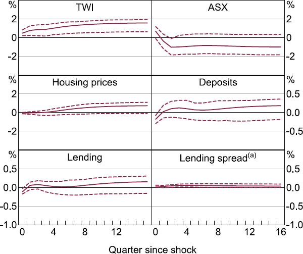
Notes:
Dashed lines show 68 per cent confidence interval.
(a) Spread between average lending rates and three-month bank bill swap rate.
References
Aastveit KA, HC Bjørnland and LA Thorsrud (2016), ‘The World Is Not Enough! Small Open Economies and Regional Dependence’, The Scandinavian Journal of Economics, 118(1), pp 168–195.
Anaya P, M Hachula and CJ Offermanns (2017), ‘Spillovers of U.S. Unconventional Monetary Policy to Emerging Markets: The Role of Capital Flows’, Journal of International Money and Finance, 73(Part B), pp 275–295.
Andrews D and M Kohler (2005), ‘International Business Cycle Co-movements through Time’, in C Kent and D Norman (eds), The Changing Nature of the Business Cycle, Proceedings of a Conference, Reserve Bank of Australia, Sydney, pp 188–219.
Atkin T and J Harris (2023), ‘Foreign Currency Exposure and Hedging in Australia’, RBA Bulletin, March.
Avdjiev S, V Bruno, C Koch and HS Shin (2019), ‘The Dollar Exchange Rate as a Global Risk Factor: Evidence from Investment’, IMF Economic Review, 67(1), pp 151–173.
Avdjiev S, RN McCauley and HS Shin (2015), ‘Breaking Free of the Triple Coincidence in International Finance’, BIS Working Papers No 524.
Bai J and S Ng (2002), ‘Determining the Number of Factors in Approximate Factor Models’, Econometrica, 70(1), pp 191–221.
Bai J and S Ng (2013), ‘Principal Components Estimation and Identification of Static Factors’, Journal of Econometrics, 176(1), pp 18–29.
Barcelona WL, D Cascaldi-Garcia, JJ Hoek and E Van Leemput (2022), ‘What Happens in China Does Not Stay in China’, Board of Governors of the Federal Reserve System International Finance Discussion Paper No 1360.
Bäurle G, M Gubler and DR Känzig (2017), ‘International Inflation Spillovers – The Role of Different Shocks’, Swiss National Bank Working Papers 7/2017.
Baxter M and MA Kouparitsas (2005), ‘Determinants of Business Cycle Comovement: A Robust Analysis’, Journal of Monetary Economics, 52(1), pp 113–157.
Beckers B (2020), ‘Credit Spreads, Monetary Policy and the Price Puzzle’, RBA Research Discussion Paper No 2020-01.
Beganau J, M Piazzesi and M Schneider (2015), ‘Banks' Risk Exposures’, NBER Working Paper No 21334.
Bellrose K and D Norman (2019), ‘The Nature of Australian Banks' Offshore Funding’, RBA Bulletin, December.
Bernanke BS, J Boivin and P Eliasz (2005), ‘Measuring the Effects of Monetary Policy: A Factor-augmented Vector Autoregressive (FAVAR) Approach’, The Quarterly Journal of Economics, 120(1), pp 387–422.
Brassil A (2022), ‘The Consequences of Low Interest Rates for the Australian Banking Sector’, RBA Research Discussion Paper No 2022-08.
Brischetto A and G Voss (1999), ‘A Structural Vector Autoregression Model of Monetary Policy in Australia’, RBA Research Discussion Paper No 1999-11.
Buch CM, M Bussierè, L Goldberg and R Hills (2019), ‘The International Transmission of Monetary Policy’, Journal of International Money and Finance, 91, pp 29–48.
Bullock M (2017), ‘Big Banks and Financial Stability’, Address given to the Melbourne Institute and The Australian Economic and Social Outlook Conference 2017 ‘New Directions in an Uncertain World’, Melbourne, 20–21 July.
Cecchetti S, T Mancini-Griffoli and M Narita (2017), ‘Does Prolonged Monetary Policy Easing Increase Financial Vulnerability?’, IMF Working Paper No WP/17/65.
Cornell WB and JK Dietrich (1978), ‘The Efficiency of the Market for Foreign Exchange under Floating Exchange Rates’, The Review of Economics and Statistics, 60(1), pp 111–120.
Croitorov O, M Giovannini, S Hohberger, M Ratto and L Vogel (2020), ‘Financial Spillover and Global Risk in a Multi-region Model of the World Economy’, Journal of Economic Behavior & Organization, 177, pp 185–218.
Davis K (2011), ‘The Australian Financial System in the 2000s: Dodging the Bullet’, in H Gerard and J Kearns (eds), The Australian Economy in the 2000s, Proceedings of a Conference, Reserve Bank of Australia, Sydney, pp 301–348.
Dedola L, G Rivolta and L Stracca (2017), ‘If the Fed Sneezes, Who Catches a Cold?’, Journal of International Economics, 108(Supplement 1), pp S23–S41.
Department of Foreign Affairs and Trade (2021a), ‘Statistics on Who Invests in Australia’, DFAT website, viewed 6 December 2024. Available at <https://webarchive.nla.gov.au/awa/20211214032353/https:/www.dfat.gov.au/trade/resources/investment-statistics/statistics-on-who-invests-in-australia>.
Department of Foreign Affairs and Trade (2021b), Trade and Investment at a Glance 2021, Department of Foreign Affairs and Trade, Barton.
Donovan B and A Gorajek (2011), ‘Developments in the Structure of the Australian Financial System’, RBA Bulletin, June, pp 29–40.
Dungey M (2001), ‘International Shocks and the Role of Domestic Policy in Australia’, Australian National University, Centre for Economic Policy Research Discussion Paper No 443.
Fitzpatrick R, C Shaw and A Suthakar (2022), ‘Developments in Banks' Funding Costs and Lending Rates’, RBA Bulletin, March.
Frenkel JA and A Razin (1987), ‘The Mundell-Fleming Model: A Quarter Century Later’, NBER Working Paper No 2321.
Georgiadis G (2015), ‘Determinants of Global Spillovers from US Monetary Policy’, ECB Working Paper No 1854.
Georgiadis G (2017), ‘To Bi, or Not to Bi? Differences between Spillover Estimates from Bilateral and Multilateral Multi-country Models’, Journal of International Economics, 107, pp 1-18.
Georgiadis G and M Jančoková (2020), ‘Financial Globalisation, Monetary Policy Spillovers and Macro-modelling: Tales from 1001 Shocks’, Journal of Economic Dynamics and Control, 121, Article 104025.
Gourinchas P-O, H Rey and M Sauzet (2019), ‘The International Monetary and Financial System’, Annual Review of Economics, 11, pp 859-893.
Greenwood-Ninmo M, VH Nguyen and Y Shin (2021), ‘Measuring the Connectedness of the Global Economy’, International Journal of Forecasting, 37(2), pp 899-919.
Guttmann R, K Hickie, P Rickards and I Roberts (2019), ‘Spillovers to Australia from the Chinese Economy’, RBA Bulletin, June.
Ha J (2021), ‘Financial Market Spillovers of U.S. Monetary Policy Shocks’, Review of International Economics, 29(5), pp 1221-1274.
Ha J, MA Kose, C Otrok and ES Prasad (2020), ‘Global Macro-financial Cycles and Spillovers’, NBER Working Paper No 26798.
Hartigan L and M Wright (2021), ‘Financial Conditions and Downside Risk to Economic Activity in Australia’, RBA Research Discussion Paper No 2021-03.
Hoffmann P, S Langfield, F Pierobon and G Vuillemey (2019), ‘Who Bears Interest Rate Risk?’, The Review of Financial Studies, 32(8), pp 2921-2954.
Iacoviello M and G Navarro (2019), ‘Foreign Effects of Higher U.S. Interest Rates’, Journal of International Money and Finance, 95, pp 232-250.
Jääskelä J and P Smith (2011), ‘Terms of Trade Shocks: What are They and What Do They Do?’, RBA Research Discussion Paper No 2011-05.
Johnson C (2022), ‘Trends in Australian Banks' Bond Issuance’, RBA Bulletin, September.
Justiniano A and B Preston (2010), ‘Can Structural Small Open-economy Models Account for the Influence of Foreign Disturbances?’, Journal of International Economics, 81(1), pp 61-74.
Kamber G and B Wong (2020), ‘Global Factors and Trend Inflation’, Journal of International Economics, 122, Article 103265.
Karagedikli Ö and LA Thorsrud (2010), ‘Shocked by the World! Introducing the Three Block Open Economy FAVAR’, Paper presented at the Reserve Bank of New Zealand conference ‘Transmission of International Shocks to Open Economies 2010’, Wellington, 16-17 December.
Kearns J, A Schrimpf and FD Xia (2023), ‘Explaining Monetary Spillovers: The Matrix Reloaded’, Journal of Money, Credit and Banking, 55(6), pp 1535-1568.
Kent C (2019), ‘The Usual Transmission – Monetary Policy and Financial Conditions’, Address to Finance and Treasury Association, Sydney, 13 August.
Lancaster D and P Tulip (2015), ‘Okun's Law and Potential Output’, RBA Research Discussion Paper No 2015-14.
Liu P (2008), ‘The Role of International Shocks in Australia's Business Cycle’, RBA Research Discussion Paper No 2008-08.
Lowe P and L Ellis (1997), ‘The Smoothing of Official Interest Rates’, in P Lowe (ed), Monetary Policy and Inflation Targeting, Proceedings of a Conference, Reserve Bank of Australia, Sydney, pp 286–312.
Lütkepohl H (2007), New Introduction to Multiple Time Series Analysis, Reprint, Springer, Berlin.
Manalo J, D Perera and D Rees (2014), ‘Exchange Rate Movements and the Australian Economy’, RBA Research Discussion Paper No 2014-11.
Mendoza EG (1991), ‘Real Business Cycles in a Small Open Economy’, The American Economic Review, 81(4), pp 797–818.
Miranda-Agrippino S and H Rey (2020), ‘U.S. Monetary Policy and the Global Financial Cycle’, The Review of Economic Studies, 87(6), pp 2754–2776.
Mumtaz H and P Surico (2009), ‘The Transmission of International Shocks: A Factor-augmented VAR Approach’, Journal of Money, Credit and Banking, 41(s1), pp 71–100.
Nimark K (2007), ‘A Structural Model of Australia as a Small Open Economy’, RBA Research Discussion Paper No 2007-01.
Pilbeam K (1992), International Finance, Macmillan Texts in Economics, Macmillan Press Ltd, Houndmills.
RBA (Reserve Bank of Australia) (2000), ‘Statement by the Governor, Mr Ian Macfarlane: Monetary Policy’, Media Release No 2000-08, 5 April.
RBA (2009a), Statement on Monetary Policy, February.
RBA (2009b), Statement on Monetary Policy, November.
RBA (2015), ‘Box A: The Effects of Changes in Iron Ore Prices’, Statement on Monetary Policy, February, pp 13–15.
RBA (2020), ‘The Exchange Rate and the Reserve Bank's Role in the Foreign Exchange Market’, Market Operations, July, viewed 6 December 2024.
Rees D, D Lancaster and R Finlay (2014), ‘A State-space Approach to Australian GDP Measurement’, RBA Research Discussion Paper No 2014-12.
Schnabel I and C Seckinger (2019), ‘Foreign Banks, Financial Crises and Economic Growth in Europe’, Journal of International Money and Finance, 95, pp 70–94.
Stock JH and MW Watson (2002), ‘Macroeconomic Forecasting Using Diffusion Indexes’, Journal of Business & Economic Statistics, 20(2), pp 147–162.
Stock JH and MW Watson (2016), ‘Dynamic Factor Models, Factor-augmented Vector Autoregressions, and Structural Vector Autoregressions in Macroeconomics’, in JB Taylor and H Uhlig (eds), Handbook of Macroeconomics: Volume 2A, Handbooks in Economics, Elsevier, Amsterdam, pp 415–525.
Tillmann P (2016), ‘Unconventional Monetary Policy and the Spillovers to Emerging Markets’, Journal of International Money and Finance, 66, pp 136–156.
Vasishtha G and P Maier (2013), ‘The Impact of the Global Business Cycle on Small Open Economies: A FAVAR Approach for Canada’, The North American Journal of Economics and Finance, 24, pp 191–207.
Yamamoto Y (2019), ‘Bootstrap Inference for Impulser Response Functions in Factor-augmented Vector Autoregressions’, Journal of Applied Econometrics, 34(2), pp 247–267.
Copyright and Disclaimer Notice
RP Data Pty Ltd trading as CoreLogic Asia Pacific Disclaimer Notice
This publication contains data, analytics, statistics, results and other information licensed to the Reserve Bank of Australia by RP Data Pty Ltd trading as Corelogic Asia Pacific (CoreLogic Data).
© Copyright 2024. RP Data Pty Ltd trading as Corelogic Asia Pacific (CoreLogic) and its licensors are the sole and exclusive owners of all rights title and interest (including intellectual property rights) subsisting in the Corelogic Data reproduced in this publication. All rights reserved.
The CoreLogic Data provided in this publication is of a general nature and should not be construed as specific advice or relied upon in lieu of appropriate professional advice.
While CoreLogic uses commercially reasonable efforts to ensure the CoreLogic data is current, CoreLogic does not warrant the accuracy, currency or completeness of the CoreLogic Data and to the full extent permitted by law excludes all loss or damage howsoever arising (including through negligence) in connection with the Corelogic Data.
Acknowledgements
We are grateful to Matthew Read for his feedback and technical assistance. Thank you to Shayan Omidi, Sam Pordeli, Claire Johnson, Joost Bats, Tim Atkin and Jacob Harris for their help obtaining data and graphs. We would also like to thank Nick Stenner, James Morley, Jeremy Lawson, Anthony Brassil, Sarah Hunter and RBA seminar and ER Coffee participants for their helpful feedback and suggestions. These are the views of the authors and not the Reserve Bank of Australia. Any remaining errors are our own.
Footnotes
‘Small’ in the sense that domestic economic shocks are unlikely to affect the world economy at large (Mendoza 1991). [1]
Specifically, a small-scale VAR, especially a bilateral VAR, may not fully capture certain shocks – for example, a bilateral VAR with the United States as the foreign block may miss shocks originating in Asia that may affect Australia more acutely (Georgiadis 2017). [2]
Under different specifications, however, such as just using the United States as the foreign block in a VAR, this buffering role is not quite as apparent, particularly on CPI (see Section 4). [3]
We include Australian variables directly in the FAVAR rather than modelling the Australian economy via a factor model of a large suite of Australian variables. This allows foreign factors to affect Australian variables directly, rather than only through their common variation with estimated domestic factors. [4]
FAVARs can also be estimated in a single stage using maximum likelihood methods, as in Hartigan and Wright (2021). We apply the two-stage approach for simplicity, as in most applications the two methods do not seem to produce significantly different results (Stock and Watson 2016). [5]
This likely underestimates the proportion of total investment from these countries, as some investment that originates in these countries may be recorded as originating from an intermediate country (such as a tax haven). [6]
The choice of transformations is supported by Dickey-Fuller tests. [7]
We used quarter-end to align the timing of monthly data with some quarterly data that is only available as quarter-ended. [8]
Our main results are robust to estimating the model starting from 1993 to align with the inflation-targeting period. [9]
The criterion determines the optimal number of factors based on the marginal added variation explained relative to a penalty term to ensure parsimony. Considering the range of sectors (real and financial) and different geographic regions in the global panel, the fact that three factors alone capture around 30 per cent of variation in the data suggests that the factors are indeed capturing important global information. [10]
For the main results of the paper, we estimate the factors freely across categories of variables (e.g. activity, prices) rather than estimating the factors within categories as in Mumtaz and Surico (2009). We choose this purely data-driven approach to estimating the factors to maximise the common variation in the global data explained by the factors and because we do not aim to identify particular types of foreign shocks. While restricting the estimation of factors as in Mumtaz and Surico (2009) could aid interpretation when paired with further identifying assumptions, the additional restriction of estimating factors for each category separately would reduce the common variation captured by the global factors under this approach. That said, our results are robust to estimating factors within blocks of categories. [11]
Global variables include global financial indices and globally traded commodities such as oil (see Appendix A). [12]
Our results are also robust to using trimmed mean CPI instead of headline and the real TWI instead of the nominal TWI. The proportion of variation explained in the trimmed mean CPI is very similar to that for headline CPI, and the proportion of variation explained for the real TWI is overall similar, but slightly higher than for the nominal TWI. [13]
We apply a residual-based bootstrap with a standard percentile interval, as described in Lütkepohl (2007). Consistent with Bernanke et al (2005), we do not account for uncertainty in our factor estimates. Yamamoto (2019) suggests that this appropriate in our case, where the number of variables is sufficiently large relative to the length of the sample. [14]
The difference in the FEV explained between the TWI and the other variables is statistically significant over the first few quarters. Towards the end of the horizon, however, only the difference between the lower FEV explained for real GDP compared to the higher FEV explained for other variables is statistically significant. [15]
Kamber and Wong (2020) find that foreign shocks explain a larger share of more than 50 per cent of the variation in cyclical inflation around its trend (the ‘inflation gap’) for Australia and other advanced economies. Their sample, however, starts in 1985, and therefore covers a longer period of high and variable inflation than our sample. Consistent with this, they also find that commodity price shocks explain much of the variation in the inflation gap. [16]
As an historical example, Governor Ian Macfarlane (RBA 2000) in a monetary policy statement suggested that a depreciation in the exchange rate pointed to the need for monetary adjustment in order to offset potential impacts on domestic inflation. Impulse responses in Figures 12 and C2 to C6 provide further evidence that the cash rate and exchange rate indeed act as buffers to the foreign shocks captured by our factors. [17]
The US block in this example includes differenced federal funds rate and 10-year Treasury yield, as well as log-differenced real GDP, CPI, stock prices (NYSE composite index), and WTI oil. [18]
Our results are robust to directly including the global financial cycle measure of Miranda-Agrippino and Rey (2020) in the foreign block. This does not increase the proportion of variation explained by foreign shocks in any variable, nor does adding major trading partner growth directly, suggesting that our foreign factors adequately capture the main sources of variation in the foreign panel. [19]
IRFs from shocks to the first and second factors are shown in Appendix C. [20]
We do not include Chinese banks in these top 50 banks due to the idiosyncrasies of China's state-dominated banking system. [21]
Though this could also reflect the greater proportional exposures of global banks to currencies that appreciated in 2021 compared to Australian banks. [22]