Research Discussion Paper – RDP 2024-07 How Do Households Form Inflation and Wage Expectations?
1. Introduction
Inflation expectations play a crucial role in modern macroeconomic models and monetary policymaking. This is because inflation expectations are thought to play an important role in wage and price setting, and a growing literature has found a causal link between inflation expectations and household and firm behaviour (e.g. Coibion et al 2023). More generally, the ability of central banks to influence and anchor expectations via credible inflation targets is widely credited for moving economies from the Great Inflation of the 1960s and 1970s to the Great Moderation of the 1980s and 1990s (Bernanke 2004; Bordo and Orphanides 2013).
There is also a growing but relatively small literature examining the formation of wage expectations. Understanding the formation of wage expectations is important as wages are a key component of households' incomes and firms' costs. And the link between inflation and wages expectations can be extremely important. For example, as inflation rises workers may want to maintain the real purchasing power of their labour income, and so wage and inflation expectations may be mechanically linked. To the extent that this feeds into higher prices, this can put further upwards pressure on prices and amplify the effects of supply or other shocks. Thankfully, recent work suggests that the extent to which this amplification leads to a spiralling of wages and prices is limited in advanced economies (Alvarez et al 2022).
In this paper we add to this literature by examining the formation of short-term wage and inflation expectations in Australia using the Melbourne Institute Consumer Survey, applying common approaches and frameworks, including that of Brassil, Gibbs and Ryan (forthcoming), to both expectations. We document several stylised facts:
- There is a negative relationship between conditions/spending intentions and expected inflation, but a positive one between conditions/spending intentions and wages.
- The contemporaneous relationship between wages expectations and inflation expectations is relatively weak.
- Estimated monetary policy shocks (an example of a demand shock) have a limited effect on expectations.
- Oil price shocks (an example of a supply shock) tend to raise inflation expectations and lead to (if anything) a decline in expected real wages.
- Inflation expectations appear to be more backward looking and based on past inflation, particularly for lower income households, while wages expectations appear more forward looking and based on a broader information set.
- Households appear to overweight past movements in certain prices, particularly fuel prices, in their inflation expectations.
These findings paint a picture of households having a somewhat ‘supply-side’ view of inflation, at least in the short term, but a more ‘demand-side’ view of wages, consistent with Jain, Kostyshyna and Zhang (2022). One potential explanation for this may be the outsized role of fuel prices in consumers' inflation expectations. If fuel prices are (perceived to be) primarily driven by supply shocks, this could help explain the supply-side view. That said, the overall estimated ‘additional’ effect of fuel prices on expectations is fairly small. An alternative explanation may be that households apply a good–bad heuristic, with inflation thought of as bad (e.g. Kamdar 2019). Relatedly, people may be focused on certain channels through which economic shocks propagate rather than others: they may focus on the effect of higher inflation, all else equal, on their real incomes, rather than the fact that higher inflation may reflect stronger economic conditions.
These findings have several related potential implications for policy. First, the findings are consistent with households potentially believing that there is relatively little trade-off between bringing down inflation and weakening economic activity, as found by Binetti, Nuzzi and Stantcheva (forthcoming). If this is the case, it may affect the central bank's ability to control inflation by influencing beliefs: if people don't believe that weaker economic conditions lead to lower inflation, communicating that policy is attempting to slow aggregate demand may not affect peoples' inflation expectations and therefore actual inflation. Moreover, if households do not believe that there is a trade-off, it may affect their willingness to face weaker conditions to bring inflation down. These issues all point to the potential benefits of effective communication and public education. Second, if people tend to associate inflation with worse economic conditions, communications about the inflation outlook may have unintended effects on households' expectations of economic conditions, as documented in Candia, Coibion and Gorodnichenko (2020). For example, communicating the importance of bringing inflation back to target following an inflationary shock could lead consumers to expect stronger economic conditions, thereby increasing the inflationary pressure.
More work is needed to draw stronger conclusions and policy lessons. For example, differentiating between some of the above explanations for the differing views of inflation and wages can help to derive more concrete recommendations for policy and communication. Unfortunately, given the difficulty in identifying the causal mechanisms that drive inflation (Read 2024), determining the causal mechanisms that drive inflation and wage expectations is likely to be even more challenging. Nevertheless, the findings generally point to the value of targeted and clear communication, as well as explanatory and educational material regarding economic channels and policy strategy.
Section 2 provides a review of the related literature. We then describe our data in Section 3, before analysing the relationship between inflation and wage expectations, and sentiment, in Section 4. Section 5 looks at the effects of various shocks on expectations, and Section 6 examines the forward- and backward-looking nature of the expectations, before Section 7 concludes.
2. Related Literature
Over the past decade or so the empirical literature on the nature and drivers of inflation expectations has grown significantly. As summarised in Weber, D'Acunto et al (2022), this literature has evolved with the growing availability of survey data (particularly respondent-level data), as well as the introduction of survey experiments. These have contributed to a large improvement in our understanding of consumers' inflation expectations, which tend to be upwardly biased, highly dispersed and uncertain, and disproportionately driven by certain salient prices.
Our paper contributes to several strands of this literature. The first is the portion exploring the relationship between sentiment and inflation expectations. Kamdar (2019), Candia et al (2020), and Andre et al (2022) document across several advanced economies a negative relationship between consumers' sentiment about the economy and their expectations for inflation. They put forward different explanations for this finding, including that households tend to make good–bad heuristic associations (i.e. inflation is bad and so is associated with bad things), that households focus more on certain channels of shock propagation, or that people focus on different sources of inflation shocks. Haidari and Nolan (2022) document a similar relationship for Australia.
Most closely related to our work, Jain et al (2022) use household-level data to look at the relationship between household-level expectations for wages and prices growth and economic conditions. As in previous work, they find a negative relationship between conditions and inflation expectations, but a positive relationship between wages and conditions. This is also evident for spending intentions.
Also related is the literature exploring the links between inflation and wage expectations. Using the same framework mentioned above, Jain et al (2022) find a relatively weak association between inflation and wage expectations. Several papers have also found similar results using experimental approaches, providing stronger causal evidence. For example, Hajdini et al (2023), using an experimental design with US consumers, find pass-through of expected inflation to income growth of only around 20 per cent, with pass-through tending to be higher for higher income individuals. As such they expect higher inflation to be associated with lower real income. Savingnac et al (2021) find similar results for firms in France. Several of these papers argue that such limited direct feedback from households' inflation expectations and perceptions to their wage expectations could limit the scope for ‘price–wage’ spirals, and more generally for amplification of supply shocks through such a mechanism.
This literature also explores the policy implications of these findings. In particular, Coibion et al (2023) provide causal evidence that providing information about higher inflation to Dutch households led them to undertake less durable spending rather than more (as would be predicted by standard theories), which they argue likely reflects lower expected real income. They argue that this highlights the potential for central bank communications aimed at moving inflation expectations to have unintended effects, and as such nuanced communication and education that draws out broader economic implications and channels may be helpful. And Binetti et al (forthcoming) find that consumers tend to believe there is little to no trade-offs between inflation and economic conditions, and that therefore there is a resistance to using monetary policy to bring down inflation by weakening aggregate demand. This naturally makes communication of a central bank's strategy more difficult.
Our paper also touches on the literature exploring the role of particular prices in determining inflation expectations. Numerous papers have highlighted that differing exposure to price signals can explain variation in consumers' inflation expectations. These differences may reflect differing consumption baskets (e.g Bürgi 2020) or variation in the specific prices people observe (e.g. Kaplan and Schulhofer-Wohl 2017; Weber, D'Acunto et al 2022; Weber, Gorodnichenko and Coibion 2022). Moreover, households tend to put higher weight on prices that appear more salient, potentially because they purchase the item more regularly (D'Acunto et al 2021), because they are more volatile (Dietrich 2024), or more generally because the price of the item is more visible to the consumer.
Finally, our paper also contributes to the broader literature trying to understand whether expectations tend to be formed using forward- or backward-looking information. We apply the framework of Brassil et al (forthcoming), which encapsulates a broad range of expectation formation mechanisms ranging from full-information rational expectations, to myopic and level-k formation (e.g. Angeletos and Lian 2018; Gabaix 2020), or adaptive learning. Beckers and Brassil (2022) apply this to union and consumer expectations. We extend their work by considering wage expectations, as well as the role of salient prices.
3. Data Description
The data we use come from the Melbourne Institute consumer survey. The survey is conducted monthly using a stratified random sample of about 1,200 households as a repeated cross-section. We use data from 1997 to mid-2024. The survey is stratified along several dimensions and weights are used to approximate the Australia population. We apply these weights for any aggregations.
We build up our measures of expectations from the unit record data, which alongside the expectations questions include various questions around socio-demographic information (e.g. sex, age, income, occupation and education), the respondent's assessment of a range of economic variables (including inflation expectations) and household finances.[1] This allows us to do individual-level analysis, as well as building up aggregate average time series for the total population and for certain demographic groups.
The two core expectations questions used in this paper are as follows:
- Inflation expectations: Consumers are asked how they expect the ‘prices of things you buy’ to change over the next year; if respondents state that prices will go ‘up’ or ‘down’, they are then asked to provide a numerical estimate for the expected change.
- Wage expectations: Consumers are asked how they expect their ‘hourly wage rate or salary or pay’ to change over the coming 12 months; if respondents state that wages will go ‘up’ or ‘down’, they are then asked to provide a numerical estimate for the expected change.
Consumers are also asked similar questions about their perceptions of price and wage changes over the past 12 months. The wages question is asked in terms of ‘total pay’, which is a slightly different concept. Though analysis suggests that people answer the two with similar notions in mind.
It is worth highlighting here that these are relatively short-term expectations. Longer-term expectations are not available in the dataset, so we cannot explore their formation.
We apply some cleaning and trimming to the expectations data. Specifically, for all analysis we trim expectations (and perceptions) below –50 per cent and above 50 per cent.
For inflation expectations, we consider two different series across the analysis. One uses the remaining data as is. The other removes rounded responses (multiples of 5) from both averages and unit-level regressions. In part this is motivated by the fact that these rounded responses contribute to a large upward bias in average reported inflation expectations relative to historical inflation outcomes (approximately 2.7 per cent over the sample). While there are other methods of removing this bias, previous research has found that changes in these rounded responses tend to reflect changes in uncertainty, with households responding in round numbers when they are uncertain about actual inflation (e.g. Binder 2017; Reiche and Meyler 2022). And while uncertainty affects decision-making, the mechanism is separate to how inflation expectations affect decisions. Removing rounded responses is therefore a more transparent and well-justified approach to removing this bias than other methods.
For wage expectations, we again consider two measures. The first uses all responses (after initial trimming). The second removes respondents reporting zero wages growth. This is because there is a large mass of people reporting zero expected or perceived wage gains – around half the sample. This is well above actual shares of wage freezes according to other sources, such as the ABS wage price index (WPI). As such, it appears that many respondents may be responding inaccurately, or reporting no gains in a very broad sense. In part this may reflect the nature of the question, where people are first asked if their wages changed, and then asked if so by how much (and if not they are recorded as zero). As we cannot differentiate ‘true’ zero expectations from these potentially imprecise responses we remove all zeros in our preferred metrics.
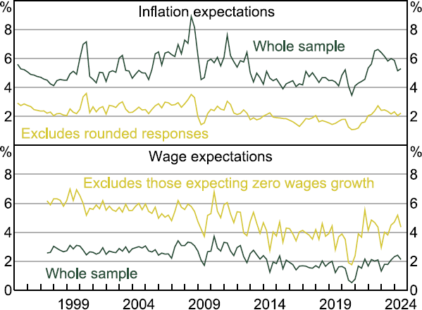
Table 1 provides some high-level summary statistics for the overall sample, and our preferred expectations metrics. Our preferred metrics end up removing around half the sample. Removing the zeros from the wage expectations data unsurprisingly lifts the mean value significantly. The full and exclusion series tend to follow quite similar patterns over time, the latter tends to be a bit smoother, especially for inflation expectations (Figure 1).
| Observations | Mean | Median | Standard deviation | Sample period | |
|---|---|---|---|---|---|
| Inflation expectations | 381,472 | 5.21 | 5.00 | 7.62 | Jan 1995–Jun 2024 |
| Inflation expectations (excluding rounded responses) | 201,009 | 2.19 | 2.00 | 3.37 | Jan 1995–Jun 2024 |
| Wages expectations | 180,788 | 2.34 | 0.00 | 7.04 | Apr 1997–Jun 2024 |
| Wages expectations (excluding zero wages growth) | 83,447 | 4.93 | 4.00 | 9.57 | Apr 1997–Jun 2024 |
|
Sources: Authors' calculations; Melbourne Institute. |
|||||
Sources: Authors' calculations; Melbourne Institute.
4. Differing Drivers of Wage and Inflation Expectations
We begin by documenting several stylised facts about the wage and inflation expectations, in terms of their correlations with sentiment about the economy, and with each other.
4.1 Wage and inflation expectations and perceptions of economic conditions
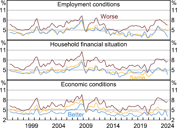
As documented by Haidari and Nolan (2022), consumers who are more pessimistic about the economic outlook tend to have higher inflation expectations. We see this when comparing average expectations over time, with households expecting better future conditions tending to have lower expectations, compared to those expecting worse future conditions (Figure 2). Similarly, when looking at the person-level correlation between expectations and sentiment we see that those with higher expectations tend to, on average, have worse expectations for future outcomes (Figure 3). Both findings are robust to removing people answering in rounded numbers.
Note: Includes rounded responses.
Sources: Authors' calculations; Melbourne Institute.
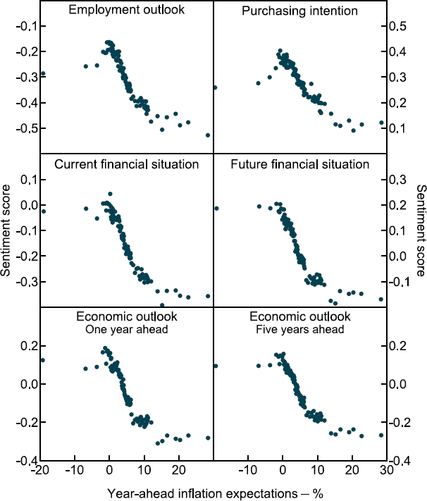
Notes: Includes rounded responses. Each panel plots a binned scatter plot of consumers' year-ahead expectations and sentiment, with those optimistic scored as 1, neutral 0 and pessimistic –1.
Sources: Authors' calculations; Melbourne Institute.
To explore these differences more concretely, we run the following regression:
where is consumer i expectation for inflation in one year's time as at time t, Xi is a number of controls for socio-economic differences, and is time fixed effects. The variables of interest Conditionsi,t are a series of questions asking the consumer about their view of the economy over the coming period, such as whether unemployment will pick up, whether economic conditions will improve or worsen, whether their financial situation will improve or worsen relative to a year ago and over the next year, or whether it is a good time to buy a large household item. We include all questions in the regression, and having separate binary dummies for ‘better’ or ‘worse’, with ‘same’ being the base case. The coefficients on these variables tell us whether positive or negative economic sentiment tends to be associated with higher or lower inflation expectations.
We again find that those expecting worse economic conditions also expect higher inflation, even once we control for potentially confounding temporal and socio-economic factors. Moreover, the finding is robust for different cohorts. While the exact magnitudes differ, the patterns are quite similar for older, middle aged and younger consumers. This suggests it does not simply reflect something about the particular historical episodes households have lived through, which has been shown to be an important determinant of people's expectations (Malmendier and Nagel 2016). Moreover, the results are also evident across the income distribution. This negative relationship is consistent with studies using data from the United States and the euro area (Kamdar 2019; Candia et al 2020).
| Full sample | Excluding rounded responses | Excluding rounded responses – by age | Excluding rounded responses High income (> $80,000) | |||
|---|---|---|---|---|---|---|
| 18–34 | 45–64 | 65+ | ||||
| Unemployment | ||||||
| More | 1.022*** | 0.427*** | 0.500*** | 0.450*** | 0.299*** | 0.365*** |
| Less | 0.008 | 0.007 | 0.041 | −0.027 | −0.032 | −0.006 |
| Economic outlook (one year ahead) | ||||||
| Good | −0.243*** | −0.142*** | −0.152*** | −0.113*** | −0.149*** | −0.100*** |
| Bad | 0.513*** | 0.181*** | 0.228*** | 0.188*** | 0.091** | 0.187*** |
| Economic outlook (five years ahead) | ||||||
| Good | −0.298*** | −0.169*** | −0.012 | −0.220*** | −0.222*** | −0.132*** |
| Bad | 0.494*** | 0.141*** | 0.199*** | 0.133*** | 0.099** | 0.144*** |
| Financial situation (one year ahead) | ||||||
| Better | 0.090*** | 0.060*** | 0.138*** | −0.002 | −0.020 | 0.070*** |
| Worse | 1.171*** | 0.637*** | 0.463*** | 0.636*** | 0.768*** | 0.610*** |
| Time to purchase large household item | ||||||
| Good | 0.047 | 0.037* | 0.264*** | −0.080*** | −0.088*** | 0.050* |
| Bad | 0.432*** | 0.142*** | 0.197*** | 0.071* | 0.103** | 0.186*** |
| R2 | 0.075 | 0.061 | 0.037 | 0.075 | 0.090 | 0.062 |
| Observations | 379,359 | 199,805 | 40,856 | 73,400 | 49,475 | 88,313 |
|
Notes: The dependent variable is households' year-ahead inflation expectations. Controls includes regional dummies, change in financial situation over last 12 months, socio-demographics (home ownership, income, education, voting preference, occupation, sex and age) and time fixed effects. Expressed relative to neutral sentiment. Regressions are unweighted. ***, ** and * denote significance at the 1, 5 and 10 per cent levels, respectively. Robust standard errors. Sources: Authors' calculations; Melbourne Institute. |
||||||
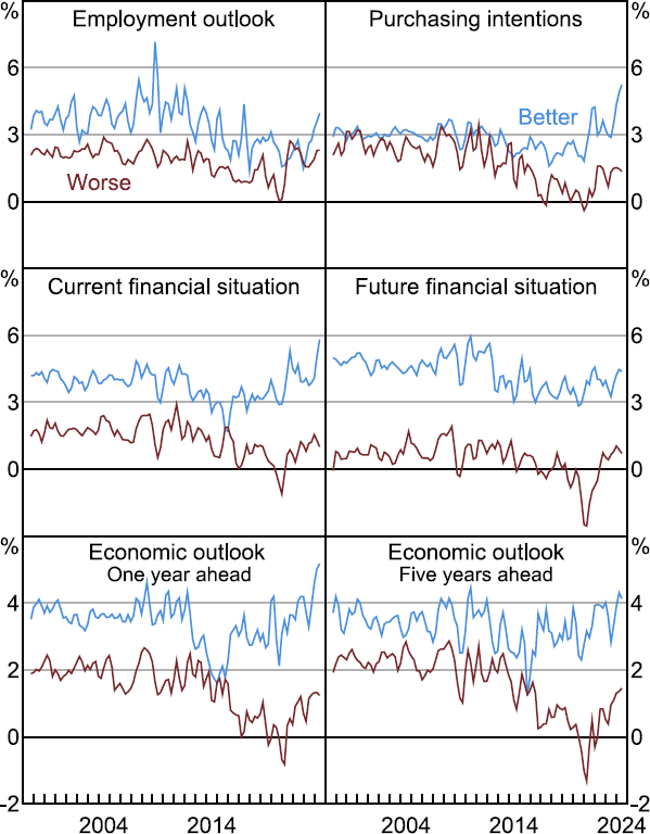
These dynamics are the opposite for wage expectations. Households that feel optimistic about the economic outlook tend, on average, to have higher wage expectations than those who expect conditions in the future to be similar or worse than they are currently (Figure 4).[2] And those individuals who expect better conditions tend to have higher wage expectations (Figure 5).
Note: Includes those expecting zero wages growth.
Sources: Authors' calculations; Melbourne Institute.
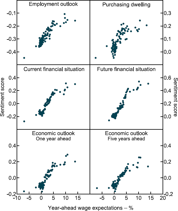
Notes: Excludes those expecting zero wages growth. Each panel plots a binned scatter plot of consumers' year-ahead wage expectations and sentiment, with those optimistic scored as 1, neutral 0 and pessimistic –1.
Sources: Authors' calculations; Melbourne Institute.
Again, this positive relationship holds once we move to the regression framework (as above but replacing inflation with wages growth) (Table 3). For example, there is a strong positive relationship between people's expectations for their financial situation and their wage growth, as might be expected. This positive relationship is again quite consistent across cohorts, though it is less evident for older cohorts, potentially as they are no longer working and so questions around their wage growth are less intuitive. Overall though, these findings are consistent with studies using data from Canada (Jain et al 2022).
| Full sample | Excluding zero wages growth | Excluding zero wages growth – by age | Excluding zero wages growth High income (> $80K) | |||
|---|---|---|---|---|---|---|
| 18–34 | 45–64 | 65+ | ||||
| Unemployment | ||||||
| More | −0.163*** | −0.405*** | −0.168 | −0.586*** | −0.179 | −0.419*** |
| Less | 0.395*** | 0.355*** | 0.513*** | 0.277* | 0.848 | 0.378*** |
| Economic outlook (one year ahead) | ||||||
| Good | 0.331*** | 0.340*** | 0.533*** | 0.152 | −0.522 | 0.388*** |
| Bad | −0.192*** | −0.334*** | −0.046 | −0.447*** | −1.016 | −0.240** |
| Economic outlook (five years ahead) | ||||||
| Good | 0.306*** | 0.341*** | 0.246 | 0.233** | 1.180* | 0.334*** |
| Bad | −0.112*** | −0.198** | −0.262 | −0.133 | −0.201 | −0.082 |
| Financial situation (one year ahead) | ||||||
| Better | 1.934*** | 2.435*** | 2.511*** | 2.391*** | 2.934*** | 2.267*** |
| Worse | −0.882*** | −2.371*** | −2.181*** | −2.498*** | −2.780*** | −2.437*** |
| Time to purchase large household item | ||||||
| Good | 0.303*** | 0.317*** | 0.403** | 0.233* | −0.515 | 0.323*** |
| Bad | −0.018 | −0.012 | 0.183 | −0.033 | −1.481* | −0.005 |
| Inflation expectations | 0.055*** | 0.113*** | 0.126*** | 0.064*** | −0.048 | 0.111*** |
| R2 | 0.071 | 0.085 | 0.075 | 0.073 | 0.112 | 0.093 |
| Observations | 165,538 | 78,356 | 23,684 | 32,178 | 2,274 | 45,999 |
|
Notes: The dependent variable is households' year-ahead wage expectations. Controls includes regional dummies, change in financial situation over last 12 months, socio-demographics (home ownership, income, education, voting preference, occupation, sex and age) and time fixed effects. Expressed relative to neutral sentiment. Regressions are unweighted. ***, ** and * denote significance at the 1, 5 and 10 per cent levels, respectively. Robust standard errors. Sources: Authors' calculations; Melbourne Institute. |
||||||
Taking these two findings together suggests that households generally associate improvements in the labour market and broader economy with higher wages growth but lower inflation. As well as being in line with Jain et al (2022), the finding is also somewhat consistent with Binetti et al (forthcoming), who find that consumers believe there are no trade-offs between inflation and economic conditions and so are resistant to the use of monetary policy to bring down inflation by weakening aggregate demand.
As discussed above, there are several potential explanations for these findings. First, it could be that households have a ‘good–bad heuristic’: they see price inflation as something bad and wage inflation as good, and so associate them with bad and good things, respectively (Kamdar 2019). It could also be that they have differing focuses on the various channels through which shocks affect outcomes. For example, they might focus on the negative effect of higher inflation on their real income (Hajdini et al 2023). Or it could reflect differing views about the nature of the shocks that drive both variables, with households tending to have a supply-side view of price inflation but a demand-side view of wage inflation (e.g. Candia et al 2020). We try to explore these explanations in more detail through the next sections.[3]
4.2 The relationship between wage and inflation expectations
As noted above, an important aspect of wage and inflation expectations is how they interact. If higher inflation outcomes or expectations feed into households' demand and expectations for wages, this can amplify the effects of economic shocks. While we cannot causally examine the relationship and pass-through between inflation and wage expectations, we can still document the reduced-form relationships in the survey. We focus on the contemporaneous relationship between inflation and wage expectations, rather than any medium-term relationships. It is possible that this may miss some pass-through if it is gradual, for example, due to differing price-setting rigidities. But given the data are a repeated cross-section and not a panel, we focus on contemporaneous relationship.
Focusing first on the aggregate time series (Figure 6), there is a moderate positive relationship between households' year-ahead wage expectations and their inflation expectations, with the two having a correlation of 0.5. This is also true of wage expectations and inflation perceptions.[4] There is also a relationship when we focus on consumer-level results (Figure 7). That said, the magnitudes suggest relatively low pass-through: the slope of a line of best fit from the individual-level scatter plots suggests a 1 percentage point increase in inflation perceptions or expectations passes through to only around an 0.1 percentage point rise in wage expectations.
This finding of low pass-through is also evident if we use a regression framework, controlling for time and other effects and focusing in on person-level variation in both variables (Table 3). Specifically, when incorporating inflation expectations into the above wage expectations regression, the coefficient on inflation expectations is very small at around 0.05–0.1. So, a 1 percentage point rise in inflation expectations would only be associated with a 0.05–0.1 percentage point rise in wage expectations.
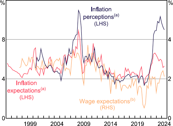
Notes:
(a) Includes rounded responses.
(b) Includes those expecting zero wages growth.
Sources: Authors' calculations; Melbourne Institute.

Notes: Excludes those expecting zero wages growth or zero inflation. Each panel plots a binned scatter plot. Line is line of best fit.
Sources: Authors' calculations; Melbourne Institute.
These findings are perhaps unsurprising given the earlier findings that suggest households have quite different views of the correlates of inflation and wage growth. They are also consistent with Jain et al (2022) and Hajdini et al (2023), who also find a small but positive pass-through from inflation expectations to expected wages growth for households in Canada and the United States respectively, and Savignac et al (2021) who find similar for firms in France. While we need to be careful about interpretation as our results are correlations, rather than causal, they do provide some evidence that there may be relatively limited direct feedback from households' inflation expectations and perceptions to their wage expectation, which could limit the scope for amplification of supply shocks through such a mechanism.[5]
That said, there are a number of other potential explanations for these findings that should temper these conclusions. For example, if supply shocks are a key driver of expectations, the natural divergence between inflation and conditions could bias down our estimate of the causal pass-through between inflation and wage expectations. Similarly, the pass-through may be gradual due to differing rigidities in price and wage setting, and our contemporaneous approach to measurement may miss this.
5. Responsiveness of Expectations to Shocks
The above results provide a number of stylised facts that suggest that inflation and wages expectations are formed somewhat differently. However, the findings are correlations, rather than causal. Moreover, they do not give us any indication of why they are formed differently.
One way to try address this is to examine how inflation and wages expectations respond to various economic shocks. As these shocks are exogenous, the findings should have a causal interpretation. Moreover, one explanation for the above findings is that supply shocks are an important driver of households' expectations, particularly their inflation expectations. Looking at the effects of supply shocks on wage and inflation expectations can help us explore this.
For this analysis we adopt a local projection regression of the following form:
where Et+h is the expectation measure h periods ahead. This is measured at the aggregate level, either across all respondents or as a microaggregate for a certain cohort. To improve estimation efficiency, we include a number of controls (inflation, GDP growth and the unemployment rate). To account for serial correlation, we include two lags of these controls, as well as two lags of the shock and left-hand side variables. We use robust standard errors. The findings are generally robust to using different lag lengths and excluding the macro controls (see Appendix A).
5.1 Expectations and monetary policy (demand) shocks
The first shock we explore is a monetary policy shock. This will essentially be a shock to aggregate demand, so standard theory would suggest that both inflation and wage expectations should fall in response to a contractionary shock.
As our monetary policy shock we use the measure outlined Beckers (2020). This is a Romer and Romer (2004)-style shock, constructed as divergences of the observed policy rate from the predictions of an estimated policy reaction function. The reaction function is a Taylor rule augmented with forecasts for economic conditions and several indicators of financial conditions. As such, it removes the anticipatory component of monetary policy by purging the changes in the policy rate of the central bank's systematic response to its own forecasts. We choose this measure as it has been shown to overcome the price puzzle. We also check robustness using high-frequency identified measures in Hambur and Haque (2024). In both cases shocks are only available for the pre-COVID-19 period.
Overall, we find very little evidence that monetary policy shocks affect households' inflation expectations in aggregate (Figure 8). Notwithstanding some volatility after around two years, inflation expectations do not appear to significantly move following a shock. This is slightly surprising given Beckers (2020) showed that these shocks do push down inflation. One explanation for this might be that expectations are well anchored, and households expect the effects of the shock to be fairly short-lived. This would be consistent with the findings in Coibion et al (2020), who find that monetary policy announcements have little effect on inflation expectations in a number of low-inflation economies. Another might be that expectations are somewhat backward looking and slow to update (consistent with our findings in Section 6), meaning expectations are slow to respond, particularly to a temporary policy shock.
As a further exercise we explore heterogeneity based on housing tenure. This is potentially interesting as we could imagine higher rates flow through to perceived costs for people with differing housing tenures quite differently. For example, even though it is not a component of the CPI, if home owners with a mortgage consider mortgage interest rates to be a component of the ‘things you buy’ (as asked by the survey), we might see expectations for this group rise after a contractionary shock. Similarly, if renters expect higher interest rates paid by their landlords to be passed onto their rents they might raise their expectations.[6] There is limited evidence of differing responses of different household types to monetary policy shocks. Despite some volatility, all show little to no change in expectations following a shock.[7]
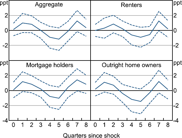
Notes: Inflation expectations exclude rounded responses. Dashed lines indicate 90 per cent confidence intervals.
Sources: Authors' calculations; Melbourne Institute.
Turning to wage expectations, we again find very limited evidence of an aggregate effect (Figure 9). In part this is unsurprising, given the estimated response of actual wages, as embodied by the WPI, is not significant.
Again, it is interesting to explore heterogeneity in this result. A particular angle of interest is heterogeneity across income groups. Previous work has shown that employment income for lower income households tends to be more responsive to the economic cycle (e.g. Coates and Ballantyne 2022). As such, we might expect expectations for lower income households to be less responsive. At the same time, lower income households may be expected to be less attentive to future conditions as they may be constrained – off their intemporal Euler equations – meaning expectations for future outcomes are less important for current decisions. Overall though, we find very little evidence that wages expectations respond for any income group.
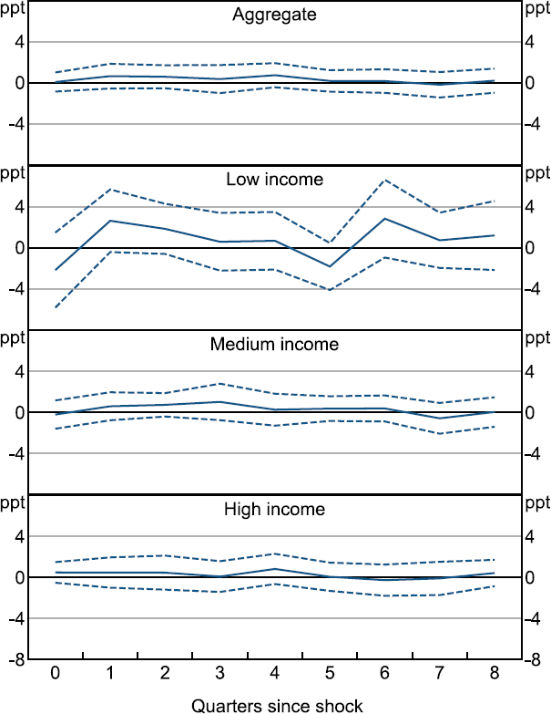
Notes: Wage expectations exclude those expecting zero wages growth. Low income defined as below $40,000, medium income as $40,000 to $100,000, and high income as above $100,000. Dashed lines indicate 90 per cent confidence intervals.
Sources: Authors' calculations; Melbourne Institute.
5.2 Expectations and oil price (supply) shocks
The second shock we explore is an oil supply shock. This is a standard supply shock that should push up inflation, but weaken economic activity. As such, if such shocks are important for households' inflation expectation formation it could help to explain the above negative association between inflation expectations and conditions.
The measure of oil supply shocks we consider is taken from Känzig (2021), which uses high-frequency changes in oil prices around OPEC announcements. We use this measure to instrument changes in domestic fuel prices in order to scale the effect to something interpretable for the Australian economy.
For this analysis we focus both on the preferred wage and inflation expectations, removing zero wages growth and rounded responses, respectively, and the full sample of responses, given it makes a moderate difference to the interpretation. We also construct a measure of real wage expectations (wage expectations less inflation expectations) to capture the perceived effect on real income, which may be better aligned to expectations for economic conditions compared to the nominal wage expectations in response to a supply shock.
Focusing first on the effect on inflation, we find that a 1 per cent supply-driven increase in the price of fuel pushes up inflation expectations by around 0.04 percentage points within the first couple of quarters removing the rounded responses (Figure 10). This is broadly in line with the fact that fuel prices make up around 4 per cent of the consumption basket. Focusing on the full sample of inflation expectations the effect is somewhat larger, at around 0.10 percentage points. For comparison, the actual effect on inflation is around 0.075 percentage points (Figure A1). So overall, the effects on inflation expectations are broadly in line with the actual effect.
That said, as discussed below in Section 6, only a moderate share of households appears to form their expectations using forward-looking information and the rate of learning from past data is quite slow, on average over time. So households' expectations are potentially a bit more responsive to oil price shocks than they are to the ‘average’ shock.
There is also some evidence that wage expectations increase following an oil price shock, before falling. This is somewhat surprising as WPI does not respond to an oil price shock (see Figure A1). The increase in wage expectations tends to be a bit smaller than the response of inflation. To see this more directly we can look at the effect on real wages. These tend to decline somewhat after the initial shock, particularly when focusing on the full sample, before rebounding.
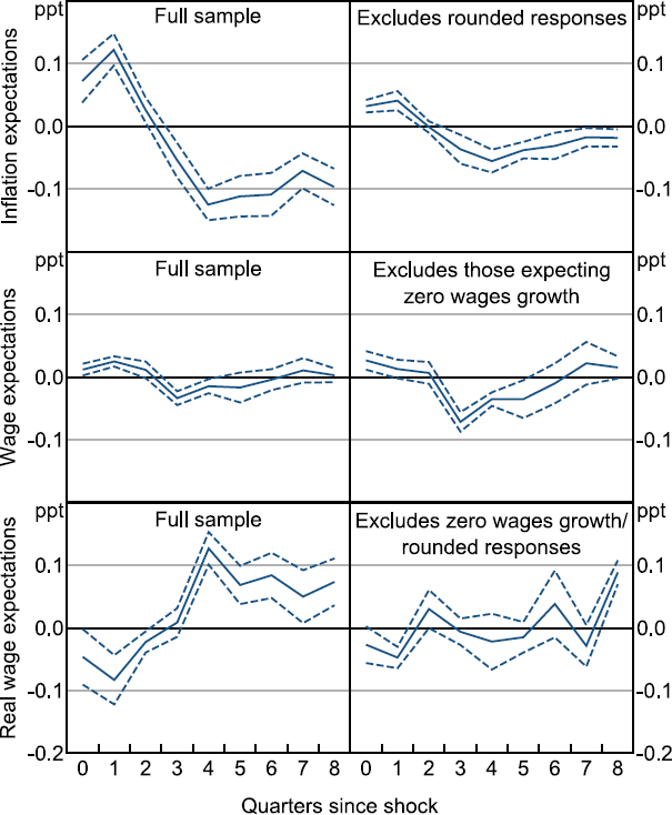
Notes: All responses outside –50 to 50 per cent are trimmed. Dashed lines indicate 90 per cent confidence intervals.
Sources: Authors' calculations; Melbourne Institute.
6. Formation of Wage and Inflation Expectations
To continue our analysis, we use a theoretical framework to understand how households form their expectations. There is an extensive literature proposing many different theories of expectation formation. We adopt the hybrid expectations framework of Brassil, Gibbs and Ryan (forthcoming, ‘BGR’) (also presented in Beckers and Brassil (2022)). This model is simple and parsimonious, while still nesting a range of plausible expectation formation behaviours. Section 6.1 introduces the framework, Section 6.2 provides baseline parameter estimates and Section 6.3 then extends the framework to incorporate a role for especially salient prices.
6.1 The BGR model and implementation
The BGR framework allows for some share of expectations to be a particular type of ‘forward-looking’ expectations known as ‘rational expectations’, while the remainder of expectations are ‘backward looking’ in the sense that they are extrapolated from observed past outcomes via a learning process. Specifically, we consider the following model for inflation expectations:
where is headline inflation, and are the average and rational inflation expectations over the next period, respectively, and is ‘learned’ expectations. The parameter is the share of expectations (or people) that are forward looking (rational). The remaining are backward looking (learned). The variable represents learners' beliefs about the persistent component of inflation, which determines their inflation expectations. The parameter g determines the rate at which these beliefs are updated given new inflation observations; the learning literature calls it the ‘gain’ parameter.[8]
Despite having only two parameters, this framework nests several common models of expectation formation, including full rational expectations , adaptive expectations , ‘myopic’ expectations models ,[9] and fixed expectations .
To implement these models we need a proxy for the rational inflation expectation and the perceived rate of inflation that learners update from . For the former we use RBA forecasts for wages and inflation.[10] For the latter we used observed headline CPI or the WPI as our base, but also explored the use of the survey measure of households' perception of past inflation or wages growth.
To estimate the model we write it in state-space form and take a maximum likelihood approach to estimate parameters, using the Kalman filter to estimate the unobserved variable . The model we estimate is:
where is our measure of one-year-ahead expectations, is one-year-ahead RBA forecasts, is year-ended CPI growth (or WPI growth or perceived outcomes), and are uncorrelated white noise error terms. We include a constant c and a dummy for the post-GFC period cGFC. They account for level differences between expectations series and outcomes, as well as the downward-level shift in some expectations series in the post-GFC period.[11] Since we have data on one-year-ahead expectations, we let them evolve according to year-ended forecast errors.
6.2 Baseline results
We first estimate the model for one-year-ahead consumer inflation expectations. We use average expectations from the Melbourne Institute survey for the dependent variable (excluding rounded responses). We have a quarterly sample from 1995:Q1 to 2024:Q2 (we use the first four observations to initialise the Kalman filter). For this baseline regression we find = 0.22 (with a 95 per cent confidence interval of 0.15-0.30) and = 0.11 (0.07-0.14) (Table 4). This suggests that around a quarter of consumer inflation expectations are forward looking, while slightly over three-quarters are backward looking. The backward-looking component incorporates around 11 per cent of observed year-ended inflation each year and so learns relatively slowly based on past outcomes.
| Sample | Standard error | Standard error | Observations | ||
|---|---|---|---|---|---|
| Baseline model | 0.22*** | 0.04 | 0.11*** | 0.02 | 114 |
| Model with rounded responses | 0.52*** | 0.06 | 0.18*** | 0.04 | 114 |
| Model with inflation perceptions | 0.27*** | 0.03 | 0.15*** | 0.03 | 95 |
| Low income | 0.21*** | 0.03 | 0.07*** | 0.02 | 114 |
| Middle income | 0.20*** | 0.05 | 0.11*** | 0.02 | 114 |
| High income | 0.26*** | 0.06 | 0.14*** | 0.03 | 114 |
| Renters | 0.20*** | 0.06 | 0.05** | 0.02 | 114 |
| Mortgagers | 0.21*** | 0.04 | 0.13*** | 0.02 | 114 |
| Owners | 0.24*** | 0.04 | 0.13*** | 0.03 | 114 |
| 18–34 years old | 0.14** | 0.06 | 0.08*** | 0.02 | 114 |
| 34–54 years old | 0.18*** | 0.06 | 0.12*** | 0.02 | 114 |
| 55+ years old | 0.36*** | 0.05 | 0.22*** | 0.04 | 114 |
| Sample from 2004 | 0.12 | 0.08 | 0.14*** | 0.02 | 76 |
| Break model (pre-2021) | 0.23*** | 0.04 | 0.12*** | 0.03 | 102 |
| Break model (post-2021 change) | 0.07 | 0.10 | −0.05 | 0.03 | 12 |
|
Notes: Model estimated per Equation (1). Includes constant and dummy for post-GFC period. ***, ** and * denote significance at the 1, 5 and 10 per cent levels, respectively. Inflation perceptions sample is 1999:Q4 to 2024:Q2. The inflation perceptions measure is an average across the months in the quarter, with rounded responses removed. In the ‘Break model’, the break is in 2021:Q3. |
|||||
We conduct a range of robustness checks around these results. First, we consider what happens if we include the rounded responses, which were excluded under the view that they may be more uncertain. Doing so does change the findings somewhat, making consumes appear more forward looking. This suggests that variation in the round responses may contain some information. Nevertheless, given the previously discussed issue with such measures we are wary of giving this finding too much credence.
Second, we use households' perceptions of inflation in place of the actual CPI. Doing so makes very little difference to the baseline results. In some senses this is surprising given the extensive evidence that households' perceptions of their own basket is a key driver of variation in household expectations. But this appears to be less important at the aggregate level, likely as the average basket should line up with the CPI basket by definition, notwithstanding any differences between how the CPI measures prices and how individuals think about those prices.
Third, we explore time variation in the relationship. In particular, we explore whether the relationships changed during the post-COVID-19 period. This is motivated by Figure 11. We see that, notwithstanding volatility in households' expectations, the baseline model has done a good job of fitting actual expectations over the sample. However, the baseline model has potentially underpredicted the recent decline in inflation expectations.
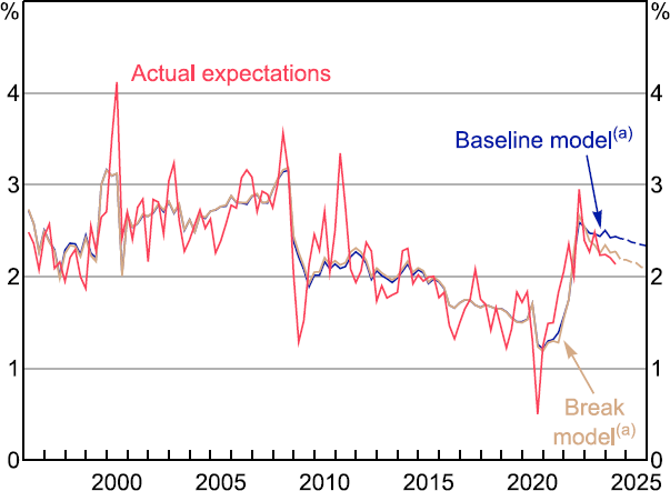
Notes:
Data are for the middle month of the quarter; excludes rounded responses.
(a) Dashed lines are out-of-sample projections for expectations using the RBA's May 2024 forecasts for headline inflation. For ‘Break model’, the parameter break occurs in 2021:Q3.
Sources: Authors' calculations; Melbourne Institute; RBA.
To account for this, we take the simple approach of allowing the model parameters to change in September 2021 (just before the pick-up in inflation). Given the short sample we do not find a significant break in the coefficients. But focusing on the point estimates, there is some evidence that expectations became more forward looking (i.e. increased) and that the learned component is less sensitive to observed outcomes (i.e. g decreased). As such the break model can better capture the sharp decline in inflation expectations observed since 2022.
The pick-up in the share of forward-looking expectations could reflect households becoming more attentive to the outlook during the period of higher inflation. Such a finding would be consistent with rational inattention models and the literature that finds consumers in high inflation countries tend to be more attentive to inflation (e.g. Coibion et al 2020). At the same time, the decline in gain parameter might reflect learners believing that the pick-up in inflation reflected transitory shocks, and so they took less signal than usual from it. It might also be that the learners who ordinarily pay more attention to past inflation (and therefore update their expectations more) were those who began to form expectations more rationally in the recent period, and so the finding could reflect a compositional shift in the nature of the learners.
Next, we consider whether the results differ across cohorts. This is interesting for several reasons. First, expectations of some groups may ‘matter’ more for economic outcomes than others. In particular, for households that are liquidity constrained expectations may have a more limited effect on their behaviour as they are consuming ‘hand-to-mouth’. Second, if there are differences across age groups this could lead to changes in aggregate relationships as the demographics of the population change. And more generally, understanding heterogeneity across groups may provide additional insights into the nature of expectations formation.
Considering this heterogeneity, we find that higher income, older and outright home owning households tend to be slightly more forward looking and learn more quickly compared to other groups. That said, the differences are numerically small. To the extent that lower income households are more likely to be liquidity constrained, and therefore off their intertemporal Euler equation, their expectations may be less influential for aggregate outcomes. So the aggregate results may slightly overstate the backward-looking nature of the expectations that affect economic outcomes.
Turning to wages, for our baseline model we find that wage expectations tend to be somewhat more forward looking, with = 0.56 (Table 5). The sensitivity of the learned component of wage expectations to lagged wage growth outcomes is similar to that for inflation expectations, with = 0.15.
| Sample | Standard error | Standard error | Observations | ||
|---|---|---|---|---|---|
| Baseline model | 0.56*** | 0.21 | 0.15 | 0.12 | 76 |
| Model with zero wage growth responses | 0.37*** | 0.10 | 0.11*** | 0.04 | 76 |
| Model with wage growth perceptions | 0.68*** | 0.21 | 0.11 | 0.08 | 76 |
|
Notes: Model estimated per Equation (1). Includes constant and dummy for post-GFC period. ***, ** and * denote significance at the 1, 5 and 10 per cent levels, respectively. |
|||||
One concern might be that the results reflect the shorter sample for which we can estimate the WPI model. However, if we re-estimate the inflation expectations model over the same sample, we still find a lower than for wage expectations. Again, using perceived wage growth in place of WPI growth does not substantially affect the results.
The model does a good job of tracking wage expectations, notwithstanding a moderate amount of volatility in the expectations measure. The model again slightly overpredicts expectations in the recent period, but the extent of the overprediction is small and short-lived (Figure 12).
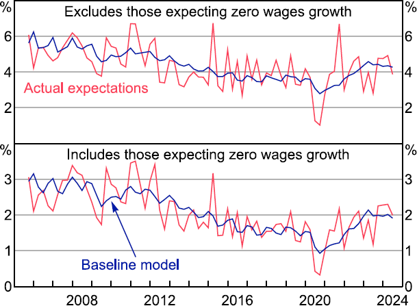
Note: Data are for the middle month of the quarter.
Sources: Authors' calculations; Melbourne Institute.
Overall, our results suggest that inflation expectations tend to be somewhat more backward looking compared to wage expectations. There are a number of different potential explanations for this, though our results cannot necessarily differentiate between them. One could be the nature of multiyear wage agreements, which mean that some households know with near certainty their wage growth over the coming year. Another could relate to our earlier findings that if households are particularly focused on supply shocks in forming their inflation expectations, but the ‘rational’ RBA forecasts place more weight on a range of shocks, inflation expectations could look less forward looking.
6.3 Salient prices or own basket?
The above results suggest that inflation expectations are formed quite differently to wage expectations. They tend to be more backward looking, placing less weight on a ‘rational’ forecast of inflation, and they potentially take a more supply-side view of inflation. To try to build on these findings we can extend the BGR framework to explore the role of ‘salient’ prices. That is, prices that play a larger role in expectation formation than is warranted by their weight in the consumption basket. These prices could be salient because households see these prices more often (e.g. D'Acunto et al 2021) or because these prices are particularly volatile so they pay more attention to them (e.g. Dietrich 2024).
To explore potential salient prices we extend the BGR model as follows:
where and are changes in some potentially salient prices series, and g1 and g2 determine the signal that backward-looking expectations take from these components (over and above their effect on headline CPI). If a component is given weight above what would be predicted based on its weight in CPI, it would have a positive and significant coefficient.
We estimate this salient prices model with a range of potentially salient prices either separately or jointly. Across specifications, the only category that was found to be robustly salient was fuel.
Table 6 compares the parameter estimates from the fuel model with the baseline model of the previous section. The rational share of expectations falls by a little but remains close to one-quarter. The gain coefficient on headline inflation falls by almost two-thirds, from 0.11 to 0.06. The coefficient on fuel is small, but fuel inflation is volatile, so can still have a significant effect on expectations.
| Baseline | Salient prices (fuel) | |
|---|---|---|
| 0.22*** (0.15–0.30) |
0.19*** (0.12–0.26) |
|
| gheadline | 0.11*** (0.07–0.14) |
0.06*** (0.02–0.11) |
| gfuel | 0.01** (0.002–0.019) |
|
| Observations | 114 | 114 |
|
Notes: Model estimated per Equation (2). Includes constant and dummy for GFC period. ***, ** and * denote significance at the 1, 5 and 10 per cent levels, respectively. Parentheses show 95 per cent confidence interval. |
||
Figure 13 shows the fitted outputs using the baseline model and the model with fuel as a salient price. While they move closely together, they have diverged slightly on occasion. For example, the model with fuel can slightly better explain the fall in expectations over 2024 as fuel prices came off their earlier high, coming down by around 0.1 percentage points more relative to the baseline model.
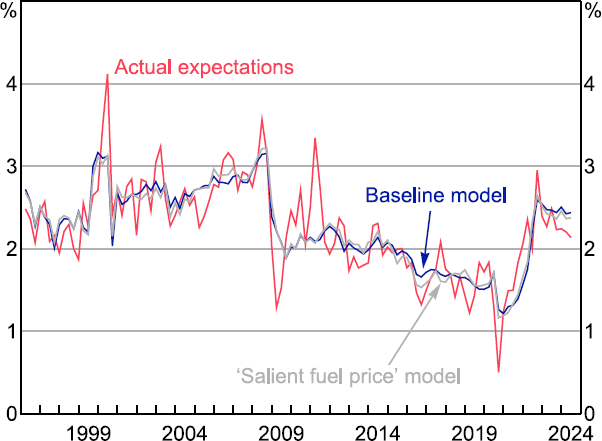
Note: Data are for the middle month of the quarter; excludes rounded responses.
Sources: Authors' calculations; Melbourne Institute.
These findings might help to explain the supply-side view that households have of inflation. Fuel price movements tend to be somewhat divorced from domestic economic conditions and tend to act as a supply shock for the Australian economy. As such, households paying attention to fuel prices may naturally have a more supply-side view of inflation. This builds on the earlier evidence showing a significant response of inflation expectations to oil supply shocks.
One further issue we explore in more detail is whether people think about inflation in a way that differs from the construction of the CPI, either because their own personal basket differs, or they think about prices of certain items (e.g. housing services) differently to how they are measured in the CPI. If, for example, home owners think about mortgage rates as a price of housing, for example, this could help to account for the negative perceived relationship between inflation and conditions (though we find no evidence of this using monetary policy shocks in Section 5.1).
While our earlier findings using inflation perceptions in the BGR model did not provide much evidence to support this argument, it may be that this simply reflected the use of aggregate measures rather than explicitly considering some non-CPI prices. As such, we explore this issue further using several different extensions:
- Including cost of living indices in place of the CPI as the signal of past inflation from which people learn, which may better align with how people perceive their costs because they include things like financing costs.
- Including measures of housing interest rates as potentially salient prices, and differentiating between mortgagors (who should respond) and renters and outright owner-occupiers (who should not).
- Taking a similar approach for rents, and comparing renters to other households.
- Including house prices, which households may perceive to be the cost of housing.
Overall, we find no strong evidence that differences between how people think about prices and their measurement in the CPI lead to different conclusions about expectation formation. Cost of living indices have less explanatory power than headline inflation in the model. Housing interest rates, unexpectedly, only affect expectations for outright owners. And rents are only relevant for mortgagors. There is some tentative evidence that households incorporate housing prices into their expectations, particularly if housing prices are included alongside some other salient prices. But this finding is less robust than the fuel finding. While further work could be considered in this space, the initial results are not promising.
7. Conclusion
Overall, the results in this paper suggest that households' short-term inflation and wage expectations are formed somewhat differently. The former appear less forward looking, and more focused on supply-side developments, while the latter are potentially more forward looking and focused on demand-side drivers of the economy. This finding is consistent with international studies, such as Jain et al (2022).
While further work is needed to draw strong conclusions, these findings do potentially present some challenges to policy. If households don't associate weakening economic conditions with lower inflation, this can make the central bank's job harder. Communicating that the central bank is raising rates to lower aggregate demand may do less to inflation expectations if people don't link weaker conditions to lower inflation. Moreover, people may be less willing to face weaker conditions to bring down inflation if they don't see a trade-off. And messaging that inflation will be higher or lower in the future may have unintended consequences if the central bank and consumers think about inflation differently.
This paper has provided some initial stylised facts and relationships. However, more work is needed to draw stronger conclusions about causal relationships, mechanisms, and therefore policy lessons. Nevertheless, the findings generally point to the value of targeted and clear communication, as well as explanatory and educational material regarding economic channels and policy strategy.
Appendix A: Regression Results
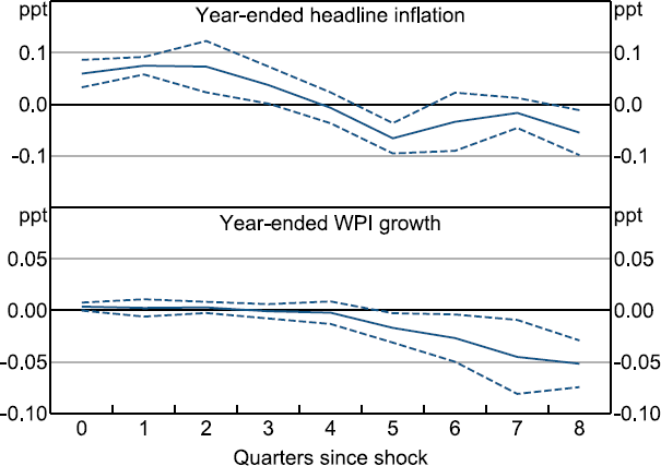
Note: Dashed lines indicate 90 per cent confidence intervals.
Sources: ABS; Authors' calculations.
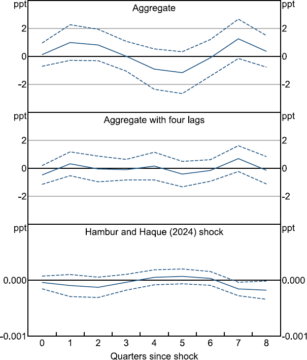
Note: Dashed lines indicate 90 per cent confidence intervals.
Sources: Authors' calculations; Melbourne Institute.
References
Alvarez J, J Bluedorn, N-J Hansen, Y Huang, E Pugacheva and A Sollaci (2022), ‘Wage-Price Spirals: What is the Historical Evidence?’, IMF Working Paper No WP/22/221.
Andre P, C Pizzinelli, C Roth and J Wohlfart (2022), ‘Subjective Models of the Macroeconomy: Evidence from Experts and Representative Samples’, The Review of Economic Studies, 89(6), pp 2958–2991.
Angeletos G-M, Z Huo and KA Sastry (2021), ‘Imperfect Macroeconomic Expectations: Evidence and Theory’, in M Eichenbaum and E Hurst (eds), NBER Macroeconomics Annual, 35, University of Chicago Press, Chicago, pp 1–86.
Angeletos G-M and C Lian (2018), ‘Forward Guidance without Common Knowledge’, The American Economic Review, 108(9), pp 2477–2512.
Beckers B (2020), ‘Credit Spreads, Monetary Policy and the Price Puzzle’, RBA Research Discussion Paper No 2020-01.
Beckers B and A Brassil (2022), ‘Inflation Expectations in Australia’, The Australian Economic Review, 55(1), pp 125–135.
Bernanke BS (2004), ‘The Great Moderation’, Remarks at the Meetings of the Eastern Economic Association, Washington DC, 20 February.
Binder CC (2017), ‘Measuring Uncertainty Based on Rounding: New Method and Application to Inflation Expectations’, Journal of Monetary Economics, 90, pp 1–12.
Binetti A, F Nuzzi and S Stantcheva (forthcoming), ‘People's Understanding of Inflation’, Journal of Monetary Economics.
Bordo MD and A Orphanides (eds) (2013), The Great Inflation: The Rebirth of Modern Central Banking, The University of Chicago Press, Chicago.
Brassil A, CG Gibbs and C Ryan (forthcoming), ‘Boundedly Rational Expectations and the Optimality of Flexible Average Inflation Targeting’, RBA Research Discussion Paper.
Bürgi C (2020), ‘Consumer Inflation Expectations and Household Weights’, The George Washington University, Department of Economics, Center of Economic Research, H. O. Stekler Research Program on Forecasting, RFP Working Paper No 2020-002.
Candia B, O Coibion and Y Gorodnichenko (2020), ‘Communication and the Beliefs of Economic Agents’, NBER Working Paper No 27800.
Coates B and A Ballantyne (2022), ‘No One Left Behind: Why Australia Should Lock in Full Employment’, Grattan Institute Report No 2022-07.
Coibion O, D Georgarakos, Y Gorodnichenko and M van Rooij (2023), ‘How Does Consumption Respond to News about Inflation? Field Evidence from a Randomized Control Trial’, American Economic Journal: Macroeconomics, 15(3), pp 109–152.
Coibion O, D Georgarakos, Y Gorodnichenko and M Weber (2020), ‘Forward Guidance and Household Expectations’, Becker Friedman Institute for Economics Working Paper No 2020-07.
D'Acunto F, U Malmendier, J Ospina and M Weber (2021), ‘Exposure to Grocery Prices and Inflation Expectations’, Journal of Political Economy, 129(5), pp 1615–1639.
Dietrich AM (2024), ‘Consumption Categories, Household Attention, and Inflation Expectations: Implications for Optimal Monetary Policy’, Journal of Monetary Economics, 147, Article 103594.
Farhi E and I Werning (2019), ‘Monetary Policy, Bounded Rationality, and Incomplete Markets’, The American Economic Review, 109(11), pp 3887–3928.
Gabaix X (2020), ‘A Behavioral New Keynesian Model’, The American Economic Review, 110(8), pp 2271–2327.
García-Schmidt M and M Woodford (2019), ‘Are Low Interest Rates Deflationary? A Paradox of Perfect-Foresight Analysis’, The American Economic Review, 109(1), pp 86–120.
Haidari Y and G Nolan (2022), ‘Sentiment, Uncertainty and Households’ Inflation Expectations', RBA Bulletin, September.
Hajdini I, ES Knotek II, J Lee, M Pedemonte, RW Rich and RS Schoenle (2023), ‘Low Passthrough from Inflation Expectations to Income Growth Expectations: Why People Dislike Inflation’, Federal Reserve Bank of Cleveland Working Paper No 22-21R.
Hambur J and Q Haque (2024), ‘Can We Use High-frequency Yield Data to Better Understand the Effects of Monetary Policy and Its Communication? Yes and No!’, Economic Record, 100(328), pp 3–43.
Hambur J, D Twohig and A Yadav (forthcoming), ‘Do Housing Investors Pass-through Changes in their Interest Costs to Rents’, RBA Bulletin.
Jain M, O Kostyshyna and X Zhang (2022), ‘How Do People View Price and Wage Inflation?’, Bank of Canada Staff Working Paper 2022-34.
Kamdar R (2019), ‘The Inattentive Consumer: Sentiment and Expectations’, Paper presented at the 2019 Annual Meeting of the Society for Economic Dynamics, St. Louis, 27–29 June.
Känzig DR (2021), ‘The Macroeconomic Effects of Oil Supply News: Evidence from OPEC Announcements’, The American Economic Review, 111(4), pp 1092–1125.
Kaplan G and S Schulhofer-Wohl (2017), ‘Inflation at the Household Level’, Journal of Monetary Economics, 91, pp 19–38.
Malmendier U and S Nagel (2016), ‘Learning from Inflation Experiences’, The Quarterly Journal of Economics, 131(1), pp 53–87.
Read M (2024), ‘Sign Restrictions and Supply-demand Decompositions of Inflation’, RBA Research Discussion Paper No 2024-05.
Reiche L and A Meyler (2022), ‘Making Sense of Consumer Inflation Expectations: The Role of Uncertainty’, ECB Working Paper Series No 2642.
Romer CD and DH Romer (2004), ‘A New Measure of Monetary Shocks: Derivation and Implications’, The American Economic Review, 94(4), pp 1055–1084.
Savignac F, E Gautier, Y Gorodnichenko and O Coibion (2021), ‘Firms’ Inflation Expectations: New Evidence from France', Banque de France Working Paper No 840.
Weber M, F D'Acunto, Y Gorodnichenko and O Coibion (2022), ‘The Subjective Inflation Expectations of Households and Firms: Measurement, Determinants, and Implications’, The Journal of Economic Perspectives, 36(3), pp 157–184.
Weber M, Y Gorodnichenko and O Coibion (2022), ‘The Expected, Perceived, and Realized Inflation of U.S. Households before and during the COVID19 Pandemic’, NBER Working Paper No 29640.
Woodford M (2019), ‘Monetary Policy Analysis When Planning Horizons Are Finite’, in M Eichenbaum and JA Parker (eds), NBER Macroeconomics Annual 2018, 33, University of Chicago Press, Chicago, pp 1–50.
Acknowledgements
Thanks to Tom Cusbert, Susan Black, Tom Rosewall, Tom Williams, Sarah Hunter and seminar participants at the Reserve Bank of Australia for comments on the paper. These are the views of the authors and not the Reserve Bank of Australia. Any remaining errors are our own. A revised version of the paper may be made available following further analysis.
Footnotes
For an analysis of households' year-ahead inflation expectations, see Haidari and Nolan (2022). [1]
This is the case for all questions related to sentiment in the survey, including employment, personal financial situation, spending (both household items and dwellings) and the general economic outlook. [2]
An alternative explanation could be that households believe that technology shocks are important economic drivers. Such shocks can cause inflation and wages to move in different directions, depending on the model of the economy one uses. However, given the ambiguity inherent in such shocks' effects, this belief seems somewhat unlikely. [3]
The correlation is about 0.4–0.5 when looking at year-ended changes but materially smaller for quarterly changes. [4]
While our results are not causal, Savignac et al (2021) and Hajdini et al (2023) use plausibly causal experimental set-ups to generate their findings. [5]
This is similar to the cost channel of monetary policy. There is little evidence of positive pass-through of landlord interest cost to rents in Australia (Hambur, Twohig and Yadav forthcoming). [6]
We also explore differences across household income levels, and find no evidence of a response for high, low or middle income households. [7]
This model can be motivated by assuming that learners believe inflation has a persistent (unit root) component and a transitory (serially uncorrelated) component, and that they estimate the persistent component from observed inflation outcomes using a steady-state Kalman filter with gain g. [8]
Here we use the term ‘myopic’ expectations models to describe a range of different frameworks in which aggregate expectations are a discounted version of the rational expectation. These models generate this aggregate property from various microfoundations, for example, cognitive discounting (Gabaix 2020), level-k reasoning (Farhi and Werning 2019; García-Schmidt and Woodford 2019), finite-horizon planning (Woodford 2019), and imperfect information (e.g. Angeletos, Huo and Sastry 2021). Some include a learning component (g = 1); others do not (g = 0). [9]
We also explored the use of market economists and Consensus Economics forecasts as proxies for the rational expectation. The results were insignificantly different. [10]
Our parameter estimates are generally robust to not including the constant and/or GFC dummy. [11]