RDP 2024-07: How Do Households Form Inflation and Wage Expectations? 6. Formation of Wage and Inflation Expectations
October 2024
- Download the Paper 1.59MB
To continue our analysis, we use a theoretical framework to understand how households form their expectations. There is an extensive literature proposing many different theories of expectation formation. We adopt the hybrid expectations framework of Brassil, Gibbs and Ryan (forthcoming, ‘BGR’) (also presented in Beckers and Brassil (2022)). This model is simple and parsimonious, while still nesting a range of plausible expectation formation behaviours. Section 6.1 introduces the framework, Section 6.2 provides baseline parameter estimates and Section 6.3 then extends the framework to incorporate a role for especially salient prices.
6.1 The BGR model and implementation
The BGR framework allows for some share of expectations to be a particular type of ‘forward-looking’ expectations known as ‘rational expectations’, while the remainder of expectations are ‘backward looking’ in the sense that they are extrapolated from observed past outcomes via a learning process. Specifically, we consider the following model for inflation expectations:
where is headline inflation, and are the average and rational inflation expectations over the next period, respectively, and is ‘learned’ expectations. The parameter is the share of expectations (or people) that are forward looking (rational). The remaining are backward looking (learned). The variable represents learners' beliefs about the persistent component of inflation, which determines their inflation expectations. The parameter g determines the rate at which these beliefs are updated given new inflation observations; the learning literature calls it the ‘gain’ parameter.[8]
Despite having only two parameters, this framework nests several common models of expectation formation, including full rational expectations , adaptive expectations , ‘myopic’ expectations models ,[9] and fixed expectations .
To implement these models we need a proxy for the rational inflation expectation and the perceived rate of inflation that learners update from . For the former we use RBA forecasts for wages and inflation.[10] For the latter we used observed headline CPI or the WPI as our base, but also explored the use of the survey measure of households' perception of past inflation or wages growth.
To estimate the model we write it in state-space form and take a maximum likelihood approach to estimate parameters, using the Kalman filter to estimate the unobserved variable . The model we estimate is:
where is our measure of one-year-ahead expectations, is one-year-ahead RBA forecasts, is year-ended CPI growth (or WPI growth or perceived outcomes), and are uncorrelated white noise error terms. We include a constant c and a dummy for the post-GFC period cGFC. They account for level differences between expectations series and outcomes, as well as the downward-level shift in some expectations series in the post-GFC period.[11] Since we have data on one-year-ahead expectations, we let them evolve according to year-ended forecast errors.
6.2 Baseline results
We first estimate the model for one-year-ahead consumer inflation expectations. We use average expectations from the Melbourne Institute survey for the dependent variable (excluding rounded responses). We have a quarterly sample from 1995:Q1 to 2024:Q2 (we use the first four observations to initialise the Kalman filter). For this baseline regression we find = 0.22 (with a 95 per cent confidence interval of 0.15-0.30) and = 0.11 (0.07-0.14) (Table 4). This suggests that around a quarter of consumer inflation expectations are forward looking, while slightly over three-quarters are backward looking. The backward-looking component incorporates around 11 per cent of observed year-ended inflation each year and so learns relatively slowly based on past outcomes.
| Sample | Standard error | Standard error | Observations | ||
|---|---|---|---|---|---|
| Baseline model | 0.22*** | 0.04 | 0.11*** | 0.02 | 114 |
| Model with rounded responses | 0.52*** | 0.06 | 0.18*** | 0.04 | 114 |
| Model with inflation perceptions | 0.27*** | 0.03 | 0.15*** | 0.03 | 95 |
| Low income | 0.21*** | 0.03 | 0.07*** | 0.02 | 114 |
| Middle income | 0.20*** | 0.05 | 0.11*** | 0.02 | 114 |
| High income | 0.26*** | 0.06 | 0.14*** | 0.03 | 114 |
| Renters | 0.20*** | 0.06 | 0.05** | 0.02 | 114 |
| Mortgagers | 0.21*** | 0.04 | 0.13*** | 0.02 | 114 |
| Owners | 0.24*** | 0.04 | 0.13*** | 0.03 | 114 |
| 18–34 years old | 0.14** | 0.06 | 0.08*** | 0.02 | 114 |
| 34–54 years old | 0.18*** | 0.06 | 0.12*** | 0.02 | 114 |
| 55+ years old | 0.36*** | 0.05 | 0.22*** | 0.04 | 114 |
| Sample from 2004 | 0.12 | 0.08 | 0.14*** | 0.02 | 76 |
| Break model (pre-2021) | 0.23*** | 0.04 | 0.12*** | 0.03 | 102 |
| Break model (post-2021 change) | 0.07 | 0.10 | −0.05 | 0.03 | 12 |
|
Notes: Model estimated per Equation (1). Includes constant and dummy for post-GFC period. ***, ** and * denote significance at the 1, 5 and 10 per cent levels, respectively. Inflation perceptions sample is 1999:Q4 to 2024:Q2. The inflation perceptions measure is an average across the months in the quarter, with rounded responses removed. In the ‘Break model’, the break is in 2021:Q3. |
|||||
We conduct a range of robustness checks around these results. First, we consider what happens if we include the rounded responses, which were excluded under the view that they may be more uncertain. Doing so does change the findings somewhat, making consumes appear more forward looking. This suggests that variation in the round responses may contain some information. Nevertheless, given the previously discussed issue with such measures we are wary of giving this finding too much credence.
Second, we use households' perceptions of inflation in place of the actual CPI. Doing so makes very little difference to the baseline results. In some senses this is surprising given the extensive evidence that households' perceptions of their own basket is a key driver of variation in household expectations. But this appears to be less important at the aggregate level, likely as the average basket should line up with the CPI basket by definition, notwithstanding any differences between how the CPI measures prices and how individuals think about those prices.
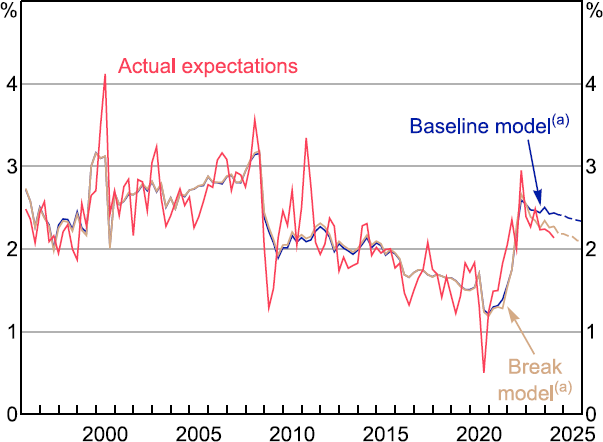
Third, we explore time variation in the relationship. In particular, we explore whether the relationships changed during the post-COVID-19 period. This is motivated by Figure 11. We see that, notwithstanding volatility in households' expectations, the baseline model has done a good job of fitting actual expectations over the sample. However, the baseline model has potentially underpredicted the recent decline in inflation expectations.

Notes:
Data are for the middle month of the quarter; excludes rounded responses.
(a) Dashed lines are out-of-sample projections for expectations using the RBA's May 2024 forecasts for headline inflation. For ‘Break model’, the parameter break occurs in 2021:Q3.
Sources: Authors' calculations; Melbourne Institute; RBA.
To account for this, we take the simple approach of allowing the model parameters to change in September 2021 (just before the pick-up in inflation). Given the short sample we do not find a significant break in the coefficients. But focusing on the point estimates, there is some evidence that expectations became more forward looking (i.e. increased) and that the learned component is less sensitive to observed outcomes (i.e. g decreased). As such the break model can better capture the sharp decline in inflation expectations observed since 2022.
The pick-up in the share of forward-looking expectations could reflect households becoming more attentive to the outlook during the period of higher inflation. Such a finding would be consistent with rational inattention models and the literature that finds consumers in high inflation countries tend to be more attentive to inflation (e.g. Coibion et al 2020). At the same time, the decline in gain parameter might reflect learners believing that the pick-up in inflation reflected transitory shocks, and so they took less signal than usual from it. It might also be that the learners who ordinarily pay more attention to past inflation (and therefore update their expectations more) were those who began to form expectations more rationally in the recent period, and so the finding could reflect a compositional shift in the nature of the learners.
Next, we consider whether the results differ across cohorts. This is interesting for several reasons. First, expectations of some groups may ‘matter’ more for economic outcomes than others. In particular, for households that are liquidity constrained expectations may have a more limited effect on their behaviour as they are consuming ‘hand-to-mouth’. Second, if there are differences across age groups this could lead to changes in aggregate relationships as the demographics of the population change. And more generally, understanding heterogeneity across groups may provide additional insights into the nature of expectations formation.
Considering this heterogeneity, we find that higher income, older and outright home owning households tend to be slightly more forward looking and learn more quickly compared to other groups. That said, the differences are numerically small. To the extent that lower income households are more likely to be liquidity constrained, and therefore off their intertemporal Euler equation, their expectations may be less influential for aggregate outcomes. So the aggregate results may slightly overstate the backward-looking nature of the expectations that affect economic outcomes.
Turning to wages, for our baseline model we find that wage expectations tend to be somewhat more forward looking, with = 0.56 (Table 5). The sensitivity of the learned component of wage expectations to lagged wage growth outcomes is similar to that for inflation expectations, with = 0.15.
| Sample | Standard error | Standard error | Observations | ||
|---|---|---|---|---|---|
| Baseline model | 0.56*** | 0.21 | 0.15 | 0.12 | 76 |
| Model with zero wage growth responses | 0.37*** | 0.10 | 0.11*** | 0.04 | 76 |
| Model with wage growth perceptions | 0.68*** | 0.21 | 0.11 | 0.08 | 76 |
|
Notes: Model estimated per Equation (1). Includes constant and dummy for post-GFC period. ***, ** and * denote significance at the 1, 5 and 10 per cent levels, respectively. |
|||||
One concern might be that the results reflect the shorter sample for which we can estimate the WPI model. However, if we re-estimate the inflation expectations model over the same sample, we still find a lower than for wage expectations. Again, using perceived wage growth in place of WPI growth does not substantially affect the results.
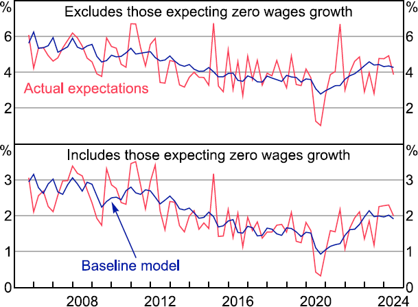
The model does a good job of tracking wage expectations, notwithstanding a moderate amount of volatility in the expectations measure. The model again slightly overpredicts expectations in the recent period, but the extent of the overprediction is small and short-lived (Figure 12).

Note: Data are for the middle month of the quarter.
Sources: Authors' calculations; Melbourne Institute.
Overall, our results suggest that inflation expectations tend to be somewhat more backward looking compared to wage expectations. There are a number of different potential explanations for this, though our results cannot necessarily differentiate between them. One could be the nature of multiyear wage agreements, which mean that some households know with near certainty their wage growth over the coming year. Another could relate to our earlier findings that if households are particularly focused on supply shocks in forming their inflation expectations, but the ‘rational’ RBA forecasts place more weight on a range of shocks, inflation expectations could look less forward looking.
6.3 Salient prices or own basket?
The above results suggest that inflation expectations are formed quite differently to wage expectations. They tend to be more backward looking, placing less weight on a ‘rational’ forecast of inflation, and they potentially take a more supply-side view of inflation. To try to build on these findings we can extend the BGR framework to explore the role of ‘salient’ prices. That is, prices that play a larger role in expectation formation than is warranted by their weight in the consumption basket. These prices could be salient because households see these prices more often (e.g. D'Acunto et al 2021) or because these prices are particularly volatile so they pay more attention to them (e.g. Dietrich 2024).
To explore potential salient prices we extend the BGR model as follows:
where and are changes in some potentially salient prices series, and g1 and g2 determine the signal that backward-looking expectations take from these components (over and above their effect on headline CPI). If a component is given weight above what would be predicted based on its weight in CPI, it would have a positive and significant coefficient.
We estimate this salient prices model with a range of potentially salient prices either separately or jointly. Across specifications, the only category that was found to be robustly salient was fuel.
Table 6 compares the parameter estimates from the fuel model with the baseline model of the previous section. The rational share of expectations falls by a little but remains close to one-quarter. The gain coefficient on headline inflation falls by almost two-thirds, from 0.11 to 0.06. The coefficient on fuel is small, but fuel inflation is volatile, so can still have a significant effect on expectations.
| Baseline | Salient prices (fuel) | |
|---|---|---|
| 0.22*** (0.15–0.30) |
0.19*** (0.12–0.26) |
|
| gheadline | 0.11*** (0.07–0.14) |
0.06*** (0.02–0.11) |
| gfuel | 0.01** (0.002–0.019) |
|
| Observations | 114 | 114 |
|
Notes: Model estimated per Equation (2). Includes constant and dummy for GFC period. ***, ** and * denote significance at the 1, 5 and 10 per cent levels, respectively. Parentheses show 95 per cent confidence interval. |
||
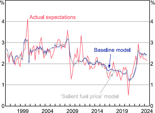
Figure 13 shows the fitted outputs using the baseline model and the model with fuel as a salient price. While they move closely together, they have diverged slightly on occasion. For example, the model with fuel can slightly better explain the fall in expectations over 2024 as fuel prices came off their earlier high, coming down by around 0.1 percentage points more relative to the baseline model.

Note: Data are for the middle month of the quarter; excludes rounded responses.
Sources: Authors' calculations; Melbourne Institute.
These findings might help to explain the supply-side view that households have of inflation. Fuel price movements tend to be somewhat divorced from domestic economic conditions and tend to act as a supply shock for the Australian economy. As such, households paying attention to fuel prices may naturally have a more supply-side view of inflation. This builds on the earlier evidence showing a significant response of inflation expectations to oil supply shocks.
One further issue we explore in more detail is whether people think about inflation in a way that differs from the construction of the CPI, either because their own personal basket differs, or they think about prices of certain items (e.g. housing services) differently to how they are measured in the CPI. If, for example, home owners think about mortgage rates as a price of housing, for example, this could help to account for the negative perceived relationship between inflation and conditions (though we find no evidence of this using monetary policy shocks in Section 5.1).
While our earlier findings using inflation perceptions in the BGR model did not provide much evidence to support this argument, it may be that this simply reflected the use of aggregate measures rather than explicitly considering some non-CPI prices. As such, we explore this issue further using several different extensions:
- Including cost of living indices in place of the CPI as the signal of past inflation from which people learn, which may better align with how people perceive their costs because they include things like financing costs.
- Including measures of housing interest rates as potentially salient prices, and differentiating between mortgagors (who should respond) and renters and outright owner-occupiers (who should not).
- Taking a similar approach for rents, and comparing renters to other households.
- Including house prices, which households may perceive to be the cost of housing.
Overall, we find no strong evidence that differences between how people think about prices and their measurement in the CPI lead to different conclusions about expectation formation. Cost of living indices have less explanatory power than headline inflation in the model. Housing interest rates, unexpectedly, only affect expectations for outright owners. And rents are only relevant for mortgagors. There is some tentative evidence that households incorporate housing prices into their expectations, particularly if housing prices are included alongside some other salient prices. But this finding is less robust than the fuel finding. While further work could be considered in this space, the initial results are not promising.
Footnotes
This model can be motivated by assuming that learners believe inflation has a persistent (unit root) component and a transitory (serially uncorrelated) component, and that they estimate the persistent component from observed inflation outcomes using a steady-state Kalman filter with gain g. [8]
Here we use the term ‘myopic’ expectations models to describe a range of different frameworks in which aggregate expectations are a discounted version of the rational expectation. These models generate this aggregate property from various microfoundations, for example, cognitive discounting (Gabaix 2020), level-k reasoning (Farhi and Werning 2019; García-Schmidt and Woodford 2019), finite-horizon planning (Woodford 2019), and imperfect information (e.g. Angeletos, Huo and Sastry 2021). Some include a learning component (g = 1); others do not (g = 0). [9]
We also explored the use of market economists and Consensus Economics forecasts as proxies for the rational expectation. The results were insignificantly different. [10]
Our parameter estimates are generally robust to not including the constant and/or GFC dummy. [11]