Research Discussion Paper – RDP 2024-05 Sign Restrictions and Supply-demand Decompositions of Infation
1. Introduction
Economists are often interested in decomposing changes in prices or quantities into contributions from shocks to supply or demand. To give a prominent example, there has been great interest in understanding how much of the surge (and subsequent decline) in inflation in many economies post COVID-19 was due to supply or demand factors.[1] Understanding the supply-demand composition of inflation is important in this context because the desired policy response may depend on the nature of the underlying shocks.
One common approach to decomposing changes in variables into contributions from different shocks is to estimate a structural vector autoregression (SVAR). Within this framework, disentangling the contributions of shocks requires making identifying assumptions. When interest is in decomposing changes in prices and quantities into contributions from supply and demand shocks, one such set of assumptions is to impose sign restrictions on the slopes of supply and demand curves or, equivalently, on the responses of prices and quantities to supply and demand shocks.[2] Economic theory typically implies that supply curves are upward sloping and demand curves are downward sloping or, equivalently, that supply shocks move prices and quantities in opposite directions, while demand shocks move them in the same direction. Hence, the main appeal of these restrictions is that they are uncontroversial. There is, however, a cost associated with relying on these relatively weak assumptions – the sign restrictions only identify a set (or range) of structural parameters, such as the slopes of the demand and supply curves (i.e. they are ‘set identifying’). In other words, there are many combinations of supply and demand curves that could explain the observed data and that are consistent with the sign restrictions. In turn, this implies that the sign restrictions can – on their own – only be used to recover a set of shock contributions or decompositions.
In this paper, I characterise the informativeness of sign restrictions when attempting to quantify the contributions of supply and demand shocks to variation in prices. I answer the question: under what conditions do these sign restrictions yield economically (un)informative decompositions of price changes? Answering this question is important because – as I discuss below – researchers have been relying on these sign restrictions when estimating the drivers of inflation. I focus on two types of decomposition. The first is the historical decomposition, which is the contribution of a particular shock to the realisation of a particular variable (or its forecast error) in a given period. For example, the historical decomposition can be used to quantify the role of supply shocks in driving the post-pandemic increase in US inflation. The second is the forecast error variance decomposition (FEVD), which is the contribution of shocks to forecast error variances. To give an example, the FEVD can be used to quantify the importance of supply shocks in driving unexpected variation in inflation over a specific forecast horizon (e.g. two years) on average over time.
This paper builds on and complements existing analyses of the use of sign restrictions in identifying supply-demand systems. In the SVAR context, Uhlig (2017) discusses the use of sign restrictions to identify the slopes of supply and demand curves given data on prices and quantities. Leamer (1981) contains a similar discussion in the context of maximum likelihood estimation of simultaneous equation systems subject to inequality constraints. Baumeister and Hamilton (2015) use a model of supply and demand to illustrate the role that the commonly used ‘uniform’ prior plays in driving Bayesian posterior inference when SVARs are identified using sign restrictions. The setting of my analysis is similar – a bivariate VAR in prices and quantities identified with sign restrictions on the slopes of supply and demand curves – but I focus on FEVDs and historical decompositions as the quantities of interest. While Baumeister and Hamilton (2015) and Uhlig (2017) use the bivariate model as a ‘toy’ example to illustrate issues associated with the use of sign restrictions, my focus on this model is motivated by its recent use empirically (as discussed below). The problem of disentangling supply and demand from data on prices and quantities is also well-studied outside of the SVAR literature and in fact was the motivating problem in the development of the instrumental variables estimator in the 1920s (e.g. Stock and Trebbi 2003).[3]
I explain that the informativeness of sign restrictions about supply-demand decompositions depends on the reduced-form correlation between price and quantity forecast errors. When this correlation is strong, the sign restrictions can allow us to draw relatively unambiguous conclusions about the contributions of shocks (in the sense that the sets of decompositions are narrow). In contrast, when this correlation is weak, the sign restrictions do not reveal much about which shock is driving variation. In the case of historical decompositions, whether the restrictions are informative also depends on the realisations of the data (or forecast errors) in the periods under consideration.
Ultimately, because the informativeness of the sign restrictions depends on features of the data, whether they allow us to draw sharp conclusions about the contributions of shocks will depend on the empirical application at hand. I estimate the contributions of supply and demand shocks to price changes in two settings.
First, I use aggregate data to estimate the contributions of aggregate supply shocks to US inflation. I follow Chang, Jansen and Pagliacci (2023) by using an SVAR that includes growth in the GDP deflator and real GDP. The SVAR is identified with sign restrictions on the slopes of aggregate supply and demand curves. Bergholt, Furlanetto and Vaccaro-Grange (2023), Bergholt et al (2024) and Giannone and Primiceri (2024) use similar models to estimate historical decompositions and/or FEVDs of inflation.[4] A feature of these papers is that, loosely speaking, they work with a single decomposition chosen from the set of decompositions that are consistent with the data and identifying restrictions. It is therefore unclear to what extent results are driven by the selection of a single, arguably arbitrary, decomposition; there are many other decompositions that are equally consistent with the identifying restrictions and the observed data.[5] Instead, I directly estimate sets of decompositions that are consistent with the sign restrictions. These sets transparently reflect what we can learn about the contributions of aggregate supply and demand shocks to inflation given the sign restrictions.
The estimated sets for the FEVD imply that aggregate supply shocks account for between zero and 80 per cent of the variance of one-step-ahead forecast errors, and between 20 and 60 per cent of the variance of forecast errors at longer horizons. Estimates of the historical decomposition suggest that supply shocks made a substantial contribution to the post-pandemic increase in inflation; for example, supply shocks are estimated to have contributed between 1.3 and 3.4 percentage points to year-ended growth in the GDP deflator in mid-2022. However, we cannot unambiguously conclude whether the increase was predominantly driven by supply or demand shocks. Moreover, the results are sensitive to whether the COVID-19 period is included in the sample used to estimate the reduced-form parameters; when the COVID-19 period is excluded, the reduced-form correlation between forecast errors in inflation and real GDP growth is close to zero, and the sign restrictions are largely uninformative about the drivers of inflation.
Second, I conduct an exercise based on disaggregated data that is motivated by an influential decomposition proposed by Shapiro (2022).[6] He estimates separate VARs for different expenditure categories of goods and services making up the personal consumption expenditures (PCE) basket and computes one-step-ahead forecast errors. Given sign restrictions on slopes of supply and demand curves, if the forecast errors have the same sign, a demand shock must have occurred, and inflation in that category is classified as ‘demand driven’. If the forecast errors have opposite signs, a supply shock must have occurred, and inflation in that category is classified as ‘supply driven’. He then takes an expenditure-weighted average of inflation in supply- and demand-driven categories to arrive at a supply-demand decomposition of aggregate inflation. A feature of this approach is that it allocates the entirety of inflation in each category to either a supply or demand shock and ignores the contributions of lagged shocks and deterministic terms. Instead, I use the historical decomposition to directly quantify the contributions of supply shocks to realised inflation within each expenditure category. The exercise therefore sheds light on the extent to which the sign restrictions underlying the decomposition in Shapiro (2022) are informative about the drivers of inflation in different expenditure categories.
I find that the sign restrictions are largely uninformative about the drivers of inflation in most expenditure categories and time periods, with some exceptions. To give an example, the sign restrictions deliver sharp decompositions of inflation in ‘food produced and consumed on farms’. Intuitively, this is because there is an extremely strong negative correlation between innovations in prices and quantities in this expenditure category, so changes in prices and quantities trace out a short-run demand curve and most variation is evidently due to supply shocks. To assess whether the disaggregated data help identify the drivers of aggregate inflation, I construct a ‘bottom-up’ decomposition of aggregate PCE inflation and compare it against the decomposition obtained when using the aggregate data directly. I find that the bottom-up decomposition tends to be substantially less informative than the aggregate decomposition, in the sense that the set of values for the contribution of supply shocks tends to be much wider.
Overall, these exercises suggest that assumptions about the signs of the slopes of supply and demand curves - on their own - may not deliver unambiguous conclusions about whether price changes are driven by shocks to supply or demand. This is the case when decomposing US inflation. Any additional assumptions inherent in selecting a single model or decomposition are likely to have a strong influence on inferences about the contributions of shocks, and these inferences may not be robust to relaxing or perturbing these additional assumptions.[7]
Outline. I describe the SVAR, historical decomposition and FEVD in Section 2 before discussing the factors that influence how informative sign restrictions are about these decompositions in Section 3. The insights from this discussion are applied in Section 4, where I estimate the contributions of supply and demand shocks to US inflation. Readers purely interested in the empirical exercises can skip to Section 4. Section 5 concludes.
Notation. I will make use of the following notation in the paper. Vectors and matrices are in bold. For a matrix X, vec(X) is the vectorisation of X, which stacks the columns of X into a vector. vech(X) is the half-vectorisation of X, which stacks the elements of X that lie on or below the diagonal into a vector. ei is the ith column of the 2 × 2 identity matrix, I2.
2. SVAR and Decompositions
This section describes a bivariate SVAR in prices and quantities, outlines a convenient alternative parameterisation of the model and introduces the structural objects of interest, including the FEVD and historical decomposition.
2.1 SVAR and orthogonal reduced form
Assume that yt = (pt, qt)′ contains data on prices pt and quantities qt, and is generated by the SVAR(p) process:
where: A0 is an invertible matrix with non-negative diagonal elements; stacks the p lags of yt; A+ = (A1,...,Ap) contains the structural coefficients on xt; and are the structural shocks, which have zero mean and identity variance-covariance matrix. For simplicity, I abstract from the inclusion of deterministic terms (e.g. a constant).
When the SVAR is set identified, it is convenient to work in the model's ‘orthogonal reduced-form’ parameterisation (e.g. Arias, Rubio-Ramírez and Waggoner 2018):
where: B = (B1,...,Bp) is a matrix of reduced-form coefficients;
is the lower-triangular Cholesky factor of the reduced-form innovation variance-covariance matrix with ut = (upt, uqt)′ = yt – Bxt; and Q is an orthonormal matrix in the space of 2 × 2 orthonormal matrices,
Let
In the absence of identifying restrictions, any orthonormal matrix Q is consistent with the second moments of the data, which are summarised by
Assume that the reduced-form parameters are such that the vector moving average
where Ch are the reduced-form impulse responses, defined by
2.2 Historical decomposition
The historical decomposition is the cumulative contribution of a particular shock to the unexpected change (i.e. forecast error) in a variable over some horizon (e.g. Antolín-Díaz and Rubio-Ramírez 2018; Baumeister and Hamilton 2018). Specifically, let Hi,j,t,t+h be the contribution of the jth shock to the unexpected change in the ith variable between periods t and t + h:
Equation (5) shows that the historical decomposition is obtained by multiplying the realisations of the structural shocks and the impulse responses to those shocks. Equation (6) represents the historical decomposition in terms of the reduced-form innovations rather than the structural shocks themselves; this representation is useful, because the reduced-form innovations are what we can recover from the data given knowledge of the reduced-form parameters.[9] To give an example, when h = 0 and i = 1, the historical decomposition represents the contribution of shock j to the one-step-ahead forecast error in pt.
Kilian and Lütkepohl (2017) define the historical decomposition as the cumulative contribution of all past realisations of a particular shock to the realisation of a particular variable in some period (see also Plagborg-Møller and Wolf (2022) or Bergholt et al (2024)). Following from the VMA
It is straightforward to show that
2.3 Forecast error variance decomposition
The FEVD of variable i at horizon h with respect to shock j is the cumulative contribution of the shock to the horizon-h forecast error variance (FEV) of variable i, expressed as a fraction of the horizon-h FEV (e.g. Kilian and Lütkepohl 2017; Baumeister and Hamilton 2018; Plagborg-Møller and Wolf 2022):
FEVDi,j,h measures by how much the FEV of variable i at horizon h is reduced by knowing the path of future realisations of structural shock j. It therefore tells us how important a particular shock is for driving unexpected variation in a particular variable over a given horizon on average over time.[10]
In the two-variable setting, knowing the contribution of one shock to the horizon-h FEV means that we know the contribution of the other shock, since FEVDi,1,h + FEVDi,2,h = 1. In what follows, I therefore focus on the contribution of the first shock to the FEV of the first variable (pt) as the object of interest, and denote this by
3. What Do Sign Restrictions Tell Us about Decompositions?
This section analytically characterises identified sets for particular structural parameters under sign restrictions on the slopes of supply and demand curves, closely following Baumeister and Hamilton (2015). I use this characterisation to discuss features of the sets of decompositions that are consistent with the restrictions, including conditions under which these sets are (un)informative about the decompositions.
3.1 Sign restrictions and identified sets
Let vech
so
where
In the absence of identifying restrictions, the identified set for
Consider imposing the following pattern of sign restrictions on
These restrictions require pt and qt to move in opposite directions in response to the first shock and in the same direction in response to the second shock. Therefore, the first shock can be interpreted as a supply shock and the second shock can be interpreted as a demand shock. Accordingly, I henceforth write
The identified set for
This identified set is identical under the following pattern of restrictions on A0:
which imply that the first equation of the SVAR describes an upward-sloping (i.e. supply) curve and the second describes a downward-sloping (i.e. demand) curve.
The structural shocks and reduced-form innovations are related via
The slopes of the supply and demand curves are the coefficients on uqt in each equation after normalising the coefficients on upt to one.
Let
It is straightforward to show that the identified set for
If the forecast errors are negatively correlated, the sign restrictions do not reveal anything about the slope of the supply curve. If the forecast errors are positively correlated, it is possible to bound the slope of the supply curve. The informativeness of these bounds depends on how strongly the forecast errors are correlated; as
Similarly, the slope of the demand curve is
and the identified set for
If the forecast errors are positively correlated, the sign restrictions reveal nothing about the slope of the demand curve. In contrast, when the forecast errors are negatively correlated, the sign restrictions generate informative bounds for the slope of the demand curve, which shrink to a point as
Figure 1 illustrates this reasoning using simulated data where the forecast errors are strongly negatively correlated. The strong negative correlation means that the forecast errors trace out the demand curve, but there is a wide range of supply curves that are consistent with the data. At one extreme, the observed forecast errors could have been generated by shifts in a vertical supply curve (corresponding to
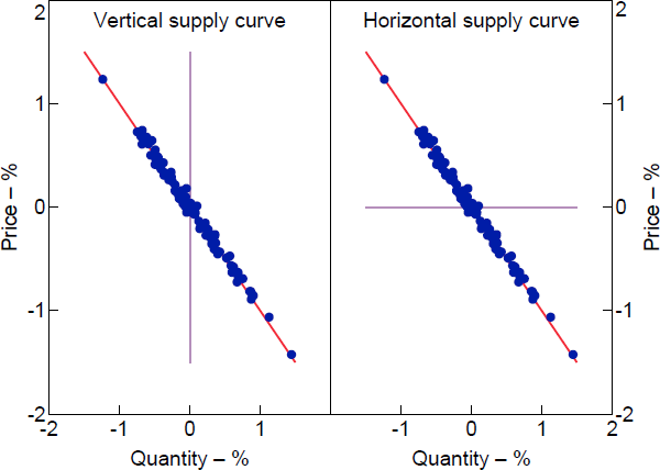
Note: Dots represent forecast errors in price and quantity; red line is demand curve; lilac line is supply curve.
3.2 Historical decomposition
In this two-variable model, we can write the historical decomposition of pt with respect to the supply shock, Ht,t+h, as a function of
where
The identified set for
where
The value of
3.2.1 Computation
3.2.2 A special case
Consider the case where interest is in the contribution of the supply shock to the one-step-ahead forecast error in pt, so h = 0. It can be shown directly that
This expression is equivalent to
The set of historical decompositions always admits ‘extreme’ contributions. When
The set of historical decompositions is uninformative when innovations are weakly correlated. If
The set of historical decompositions can be very informative when forecast errors are strongly correlated. When the forecast errors are strongly negatively correlated, they trace out the demand curve, and forecast errors predominantly reflect supply shocks. However, we learn very little about the shape of the supply curve; the same forecast errors could be generated by shocks to a supply curve that is very steep, very flat, or something in between (see Figure 1). If we observe forecast errors that are consistent with the historical negative relationship, then we can conclude that they were mainly driven by a supply shock (even though we do not know much about the shape of the supply curve), so the set of historical decompositions is narrow around the observed forecast error. Similar reasoning applies when the forecast errors are strongly positively correlated, except in that case the forecast errors trace out the supply curve and forecast errors are attributable to demand shocks.
To illustrate this case, the top panels of Figure 2 plot two potential shifts in the supply curve that could have generated a particular forecast error – specifically, a roughly 1.5 per cent fall in price and 1.5 per cent increase in quantity. The forecast error can, at one extreme, be completely explained by a shift in a vertical supply curve (top left panel) or, at the other extreme, a shift in a horizontal supply curve (top right panel). Shifts in supply curves with any intermediate slope are also compatible with the observed forecast error. Despite not knowing anything about the slope of the supply curve, the contribution of the supply shock to the forecast error in prices is pinned down to be (approximately) equal to the observed forecast error – that is, the supply shock contributed 1.5 percentage points to the unexpected decline in prices.
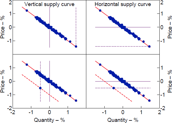
Notes: Dots represent forecast errors in price and quantity; red line is demand curve; lilac line is supply curve. Dashed lines represent shifts in supply and demand curves that could explain particular forecast errors.
But the set of historical decompositions can also be very uninformative even when forecast errors are strongly correlated. If the forecast errors are strongly negatively correlated but we observe forecast errors that depart from the historical negative relationship, the set of historical decompositions may be wide and thus economically uninformative. The bottom panels of Figure 2 illustrate the reasoning. In the left panel, a 0.5 per cent fall in both price and quantity can be explained by the combination of a negative demand shock (a downward shift in the demand curve from the solid to dashed red line) and a negative shock to a vertical supply curve (a leftward shift in the supply curve from the solid to dashed lilac line). In this case, the contribution of the supply shock to the forecast error in pt is 0.5 percentage points. Alternatively, as illustrated in the right panel, the forecast error can be explained by a combination of the same negative demand shock and a negative shock to a horizontal supply curve. In this case, the contribution of the supply shock to the forecast error in pt is −0.5 percentage points. Shifts in supply curves with slopes that lie between these two extremes are also consistent with the forecast error. The conditional identified set for the historical decomposition is therefore
3.3 Forecast error variance decomposition
We can rewrite FEVDh as
where
The identified set for
where
Computation of
3.3.1 A special case
Consider the case where interest is in the one-step-ahead FEVD of pt with respect to the supply shock, FEVD0. The contribution of
When
Echoing the analysis of the historical decomposition, the sign restrictions always admit extreme values of the FEVD. When
The sign restrictions become more informative as the magnitude of the correlation between forecast errors,
4. Supply-demand Decompositions of US Inflation
This section builds on the insights above – in terms of using the sign restrictions to set identify the contributions of supply and demand shocks – to decompose US inflation into its drivers. I conduct two exercises that relate to existing decompositions of US inflation. The first approach is based on aggregate data and relates closely to a decomposition in Chang et al (2023), as well as possessing similarities to decompositions in Bergholt et al (2023) and Giannone and Primiceri (2024). The second approach builds a bottom-up decomposition of aggregate PCE inflation using disaggregated data on different expenditure categories, and relates to the influential decomposition proposed in Shapiro (2022).
4.1 An aggregate decomposition
Using a two-variable SVAR identified via sign restrictions, Chang et al (2023) decompose inflation and real GDP growth in the United States into contributions from shocks to aggregate supply and demand. They present historical decompositions based on a single model chosen from the set of models that are consistent with the sign restrictions using the ‘median target’ criterion from Fry and Pagan (2011). In contrast, I characterise sets of decompositions that are consistent with the identifying restrictions.
The model's endogenous variables are
As above, the identifying restrictions are that aggregate supply shocks move inflation and output in opposite directions and aggregate demand shocks move them in the same direction, which is equivalent to assuming the aggregate supply curve is upward sloping and the aggregate demand curve is downward sloping. Chang et al (2023) restrict the impulse responses on impact and in the period after the shocks. To avoid making assumptions about the persistence of the effects of shocks, I impose the restrictions only on impact.
Consistent with Chang et al (2023), I estimate the contributions of both current and past supply shocks to the realisation of inflation. In the notation of Section 2.2, this means that the historical decomposition of interest is H1,t. I present decompositions of both quarterly and year-ended inflation.[20] As discussed above, it is not possible to allocate the entirety of inflation to either supply or demand shocks, because part of inflation is explained by the constant and initial conditions. For ease of presentation, Figure 3 – which presents the estimated sets of historical decompositions – plots only the part of inflation that can be explained by shocks occurring within the sample; that is, after removing the deterministic component. On average, deterministic terms contributed about 0.5 percentage points to quarterly inflation and 2 percentage points to year-ended inflation.
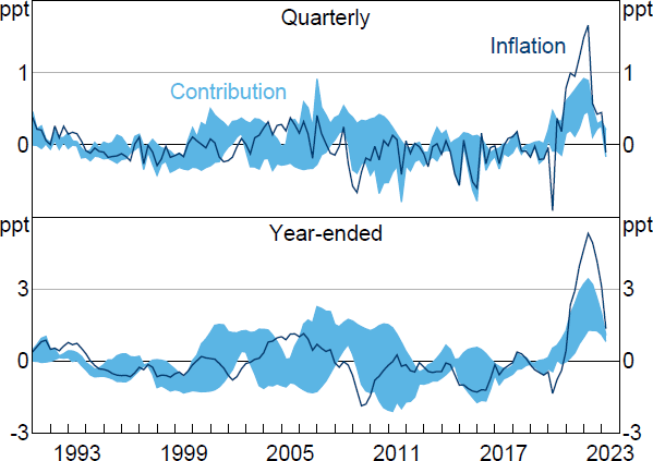
Note: Inflation is (quarterly or year-ended) growth in GDP deflator after removing contributions from constant and initial conditions.
Sources: Author's calculations; Federal Reserve Bank of St. Louis.
The correlation in the one-step-ahead forecast errors for
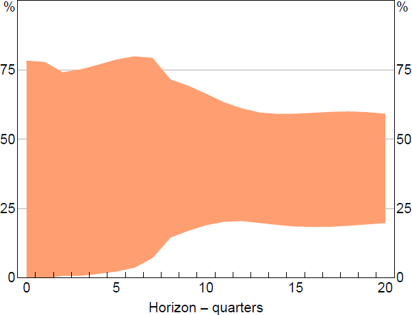
The moderate degree of correlation between the one-step-ahead forecast errors means that the identified set for the FEVD is fairly wide (Figure 4). Aggregate supply shocks are estimated to account for between zero and 78 per cent of the variance of one-step-ahead forecast errors, and between 20 and 60 per cent of the variance of forecast errors at the five-year horizon. The sign restrictions therefore do not shine much light on the drivers of aggregate inflation at short horizons, though they suggest that supply shocks make a nontrivial contribution at longer horizons.
4.1.1 Robustness
The VAR described above is estimated over a sample period that includes the COVID-19 pandemic, which is consistent with the exercise in Chang et al (2023). One may worry that the large swings in economic activity that occurred during the pandemic may unduly affect the estimates of
Re-estimating the model over this period yields an estimate for
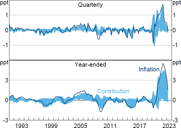
Note: Inflation is (quarterly or year-ended) growth in GDP deflator after removing contributions from constant and initial conditions.
Sources: Author's calculations; Federal Reserve Bank of St. Louis.
4.2 Disaggregated decompositions
Shapiro (2022) proposes a supply-demand decomposition of US inflation in the PCE index based on disaggregated data. The decomposition involves estimating VARs for prices and quantities consumed in different PCE expenditure groups. Given sign restrictions on the slopes of the supply and demand curves, if the price and quantity forecast errors have the same sign, a demand shock must have occurred, and the price change is classified as demand driven. If the forecast errors have opposite signs, a supply shock must have occurred, and the price change is classified as supply driven.[23] On this basis, overall inflation is decomposed into demand- and supply-driven components.
More precisely, let the superscript k index expenditure categories.
where 1(.) is the indicator function. The demand-driven component is defined similarly.[24]
A feature of this decomposition is that it allocates the entire price change in an expenditure category on the basis of contemporaneous demand or supply shocks even though these shocks could only contribute to the one-step-ahead forecast error (i.e. the ‘unexpected’ part of the price change). It therefore ignores the lagged effects of shocks and the contributions of deterministic terms. The decomposition may also misrepresent the direction in which shocks contribute to inflation. For example, if
I address these issues by directly estimating the set of historical decompositions within different expenditure categories. The concept of the historical decomposition employed is H1,t, so the effects of all past shocks are captured. The aim of the exercise is to explore the extent to which the sign restrictions allow us to learn about the contributions of supply and demand shocks within different expenditure categories. I then use the disaggregated results to construct a bottom-up decomposition of aggregate PCE inflation and compare it against a decomposition based on the aggregate PCE data. The exercise therefore speaks to whether applying the supply-demand decomposition to disaggregated data provides useful information about the contributions of supply and demand shocks to aggregate inflation relative to applying the decomposition to the aggregate data directly.
I consider 136 expenditure categories that make up the PCE data between January 1988 and September 2023.[26] Within expenditure category k, the endogenous variables are
As discussed in Section 3, the correlation between the forecast errors in prices and quantities is important in determining how informative the sign restrictions are about the slopes of supply and demand curves and thus about the contributions of shocks to inflation. The category with the smallest absolute correlation is ‘lubricants and fluids’
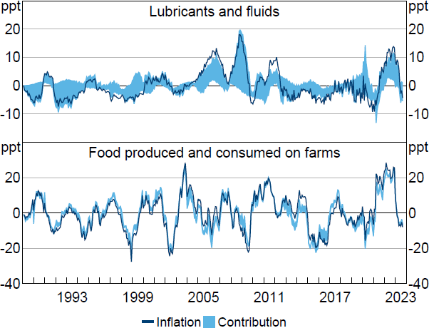
Note: Inflation is year-ended growth in price index for PCE category after removing contributions from constant and initial conditions.
Sources: Author's calculations; Bureau of Economic Analysis.
The set of historical decompositions for lubricants and fluids inflation often includes zero and the realisation of inflation itself (after removing the contribution of deterministic terms). The sets are therefore largely uninformative about whether price changes in this category are entirely driven by supply or demand shocks, which is broadly consistent with the discussion in Section 3.
In contrast, for food produced and consumed on farms, the strong negative correlation between forecast errors in prices and quantities means that the forecast errors trace out a short-run demand curve, and the contribution of supply shocks is bounded within a narrow range in most periods. To give an example, in March 2022, year-ended inflation in this expenditure category was 30.1 per cent, 28.4 percentage points of which can be explained by shocks occurring during the sample period (i.e. the contribution of deterministic components was a bit under 2 percentage points). Supply shocks are estimated to have contributed 23.9 to 25.1 percentage points to year-ended inflation in this period.
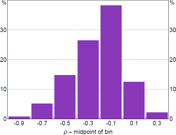
The correlation between forecasts errors tends to be reasonably weak in most other expenditure groups considered; the absolute correlations are smaller than 0.2 in about half of the categories and smaller than 0.4 in about 80 per cent of categories (Figure 7). The sign restrictions therefore tend to be fairly uninformative about the supply-demand composition of inflation outcomes within different expenditure categories.
To summarise the overall informativeness of the restrictions, I compute an expenditure-weighted average of the lower and upper bounds of the set of historical decompositions. Figure 8 presents this bottom-up decomposition of aggregate PCE inflation alongside a decomposition constructed using the aggregate PCE data directly.[28] Separately decomposing PCE inflation in disaggregated expenditure categories does not appear to generate more informative decompositions of aggregate PCE inflation relative to a direct decomposition based on the aggregate data. In fact, the bottom-up decomposition generates substantially wider sets than the aggregate decomposition; on average over the sample period, the width of the sets is 2.6 percentage points for the bottom-up decomposition compared with 1.1 percentage points for the aggregate decomposition.
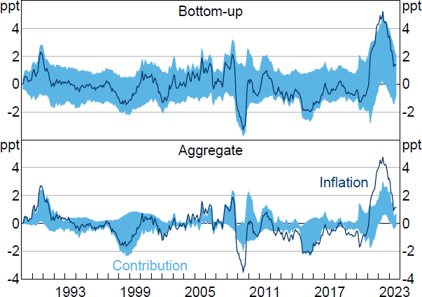
Notes: Inflation is year-ended growth in PCE price index after removing contributions from constant and initial conditions. Exercises omit two categories whose category-level VARs were unstable.
Sources: Author's calculations; Bureau of Economic Analysis.
The bottom-up decomposition clearly reveals little about the drivers of the post-pandemic surge in US inflation, admitting contributions for the supply shock ranging anywhere from around zero to the entire change (less the contribution of deterministic terms). The aggregate decomposition yields sharper conclusions; for instance, in June 2022, the aggregate decomposition suggests that supply shocks contributed between 0.7 and 3 percentage points to year-ended PCE inflation. Much like the aggregate decomposition of inflation in the GDP deflator (Section 4.1), the aggregate decomposition of PCE inflation suggests that, while supply shocks made a substantial contribution to the increase in inflation in the post-pandemic episode, the sign restrictions do not allow us to unambiguously conclude whether the increase was mostly driven by supply or demand shocks.
One reason why the bottom-up decomposition may generate less-informative decompositions of aggregate PCE inflation than using the aggregate data directly is if there is a greater degree of measurement error at finer levels of disaggregation. Intuitively, the presence of (uncorrelated) measurement error in the price and quantity data would generate one-step-ahead forecast errors that are less strongly correlated than the forecast errors that would be obtained if price and quantity were observed without error. As discussed above, weaker correlations in these forecast errors mean that the sign restrictions reveal less about the slopes of supply and demand curves and thus less about shock decompositions. Indeed, the Bureau of Economic Analysis notes that the PCE data at this level of disaggregation is of significantly lower quality than that of the higher-level categories of which they are a part, as they are more likely to be based on judgement or on less-reliable source data (Bureau of Economic Analysis 2017).[29]
As in Section 4.1.1, re-doing this exercise with an estimation sample that excludes the COVID-19 period tends to generate wider sets, both for the bottom-up and aggregate decompositions. However, it remains the case that the bottom-up decomposition yields much wider sets than the decomposition estimated using the aggregate data directly; see Appendix B.
5. Conclusion
Sign restrictions on the slopes of supply and demand curves provide an appealing avenue for identifying the contributions of supply and demand shocks to price changes because they are based on assumptions that are relatively uncontroversial. This is probably why they have been employed by researchers seeking to understand what has driven recent inflation developments. However, it is important to recognise that – on their own – these restrictions only allow us to conclude that the contributions lie within a set. In some cases, these sets may not allow us to draw unambiguous conclusions about whether price changes are mostly driven by shocks to supply or demand. In such cases, any additional assumptions that are used to select a single model or decomposition are likely to have a strong influence on assessments about which shocks are principally contributing to inflation.
While this paper focuses on estimating the contributions of supply and demand shocks to variation in prices, the discussion applies to other settings in which a bivariate system is identified using the same pattern of sign restrictions. For instance, models of search and matching in the labour market imply that equilibrium unemployment and vacancy rates are determined by the intersection of a downward-sloping Beveridge curve and an upward-sloping job creation curve (e.g. Daly et al 2012). It may therefore be appealing to use sign restrictions on the slopes of these curves to decompose variation in unemployment and vacancy rates. The analysis in this paper is useful for understanding the conditions under which such decompositions are informative.
This paper has characterised sets of decompositions, taking as given the modelling framework, which is a bivariate SVAR in prices and quantities identified via sign restrictions on the slopes of supply and demand curves. It could be useful for further work to explore what this framework identifies in terms of the underlying structure of the economy. For example, one could consider a New Keynesian model as a data-generating process and explore what the sign-restricted supply-demand framework identifies in terms of the model's underlying structural parameters and shocks.[30]
Appendix A: Inference about Decompositions
The sets of decompositions presented in Section 4 are constructed conditional on the reduced-form parameters
Standard (single prior) approaches to Bayesian inference specify a prior over
I assume a Jeffreys' prior over
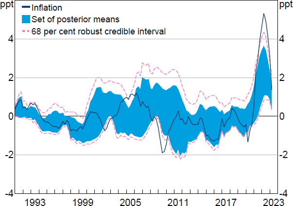
Note: Inflation is year-ended growth in GDP deflator after removing contributions from constant and initial conditions (at the posterior mean).
Sources: Author's calculations; Federal Reserve Bank of St. Louis.
Appendix B: Additional Empirical Results
This appendix explores the robustness of the decomposition of aggregate PCE inflation in Section 4.2 to excluding the COVID-19 period from the estimation sample. The VARs are estimated using a sample that runs up to 2019:M12.[36] The estimated sets tend to be wider than those obtained using the full estimation sample (Figure B1). For the decomposition based on aggregate data, these wider sets reflect that the estimated value of
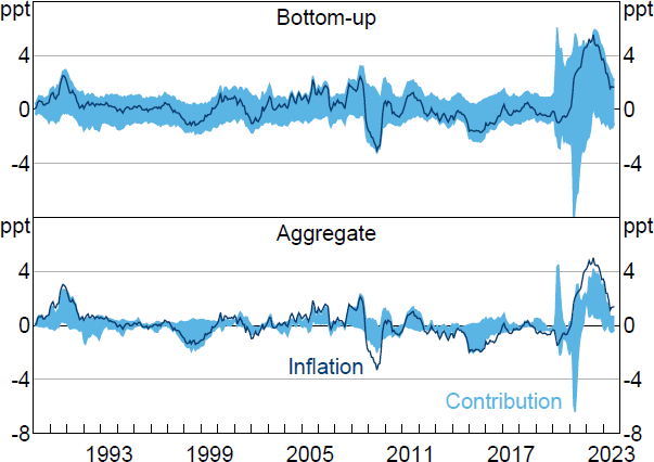
Note: Inflation is year-ended growth in PCE price index after removing contributions from constant and initial conditions.
Sources: Author's calculations; Bureau of Economic Analysis.
References
Adjemian MK, Q Li and J Jo (2023), ‘Decomposing Food Price Inflation into Supply and Demand Shocks’, Unpublished manuscript, College of Agricultural & Environmental Sciences, University of Georgia, rev 12 July 2023.
Angeletos G-M, F Collard and H Dellas (2020), ‘Business-cycle Anatomy’, The American Economic Review, 110(10), pp 3030–3070.
Antolín-Díaz J and JF Rubio-Ramírez (2018), ‘Narrative Sign Restrictions for SVARs’, The American Economic Review, 108(10), pp 2802–2829.
Arias JE, JF Rubio-Ramírez and DF Waggoner (2018), ‘Inference Based on Structural Vector Autoregressions Identified with Sign and Zero Restrictions: Theory and Applications’, Econometrica, 86(2), pp 685–720.
Aruoba SB, FX Diebold, J Nalewaik, F Schorfheide and D Song (2016), ‘Improving GDP Measurement: A Measurement-error Perspective’, Journal of Econometrics, 191(2), pp 384–397.
Bai X, J Fernández-Villaverde, Y Li and F Zanetti (2024), ‘The Causal Effects of Global Supply Chain Disruptions on Macroeconomic Outcomes: Evidence and Theory’, NBER Working Paper No 32098.
Ball LM, D Leigh and P Mishra (2022), ‘Understanding U.S. Inflation during the COVID Era’, NBER Working Paper No 30613.
Baumeister C and JD Hamilton (2015), ‘Sign Restrictions, Structural Vector Autoregressions, and Useful Prior Information’, Econometrica, 83(5), pp 1963–1999.
Baumeister C and JD Hamilton (2018), ‘Inference in Structural Vector Autoregressions When the Identifying Assumptions Are Not Fully Believed: Re-evaluating the Role of Monetary Policy in Economic Fluctuations’, Journal of Monetary Economics, 100, pp 48–65.
Beaudry P, C Hou and F Portier (forthcoming), ‘The Dominant Role of Expectations and Broad-based Supply Shocks in Driving Inflation’, in JV Leahy, MS Eichenbaum and VA Ramey (eds), NBER Macroeconomics Annual, 39, University of Chicago Press, Chicago.
Beckers B (2023), ‘Discussant Remarks by Benjamin Beckers on “Decomposing Supply and Demand Driven Inflation” by Adam Shapiro’, Discussion of ‘Decomposing Supply and Demand Driven Inflation’ presented at the annual Reserve Bank of Australia Conference on ‘Inflation’, Sydney, 25–26 September.
Beckers B, J Hambur and T Williams (2023), ‘Estimating the Relative Contributions of Supply and Demand Drivers to Inflation in Australia’, RBA Bulletin, June.
Bergholt D, F Canova, F Furlanetto, N Maffei-Faccioli and P Ulvedal (2024), ‘What Drives the Recent Surge in Inflation? The Historical Decomposition Roller Coaster’, Norges Bank Working Paper 7|2024.
Bergholt D, F Furlanetto and E Vaccaro-Grange (2023), ‘Did Monetary Policy Kill the Phillips Curve? Some Simple Arithmetics’, Norges Bank Working Paper 2|2023.
Blanchard OJ and BS Bernanke (2023), ‘What Caused the US Pandemic-era Inflation?’, NBER Working Paper No 31417.
Boissay F, F Collard, C Manea and A Shapiro (2023), ‘Monetary Tightening, Inflation Drivers and Financial Stress’, BIS Working Papers No 1155.
Braun R, A Flaaen and S Hacıoğlu Hoke (2024), ‘Supply vs Demand Factors Influencing Prices of Manufactured Goods’, Board of Governors of the Federal Reserve System, FEDS Notes, 23 February.
Bureau of Economic Analysis (2017), ‘Chapter 5: Personal Consumption Expenditures’, in ‘Concepts and Methods of the U.S. National Income and Product Accounts’, rev Dec 2023, pp 5-1–5-73.
Calvert Jump R and K Kohler (2022), ‘A History of Aggregate Demand and Supply Shocks for the United Kingdom, 1900 to 2016’, Explorations in Economic History, 85, Article 101448.
Carriero A and A Volpicella (forthcoming), ‘Max Share Identification of Multiple Shocks: An Application to Uncertainty and Financial Conditions’, Journal of Business & Economic Statistics.
Chang J-CD, DW Jansen and C Pagliacci (2023), ‘Inflation and Real GDP Growth in the U.S.— Demand or Supply Driven?’, Economics Letters, 231, Article 111274.
Chen Y and T Tombe (2023), ‘The Rise (and Fall?) of Inflation in Canada: A Detailed Analysis of Its Post-pandemic Experience’, Canadian Public Policy, 49(2), pp 197–217.
Daly MC, B Hobijn, A Şahin and RG Valletta (2012), ‘A Search and Matching Approach to Labor Markets: Did the Natural Rate of Unemployment Rise?’, Journal of Economic Perspectives, 26(3), pp 3–26.
Eickmeier S and B Hofmann (2022), ‘What Drives Inflation? Disentangling Demand and Supply Factors’, Australian National University Crawford School of Public Policy, Centre for Applied Macroeconomic Analysis, CAMA Working Paper 74/2022.
Firat M and O Hao (2023), ‘Demand vs. Supply Decomposition of Inflation: Cross-country Evidence with Applications’, IMF Working Paper No WP/23/205.
Fry R and A Pagan (2011), ‘Sign Restrictions in Structural Vector Autoregressions: A Critical Review’, Journal of Economic Literature, 49(4), pp 938–960.
Gafarov B, M Meier and JL Montiel Olea (2018), ‘Delta-method Inference for a Class of Set-identified SVARs’, Journal of Econometrics, 203(2), pp 316–327.
Giacomini R and T Kitagawa (2021), ‘Robust Bayesian Inference for Set-identified Models’, Econometrica, 89(4), pp 1519–1556.
Giacomini R, T Kitagawa and M Read (2023), ‘Identification and Inference under Narrative Restrictions’, RBA Research Discussion Paper No 2023-07.
Giannone D and GE Primiceri (2024), ‘The Drivers of Post-pandemic Inflation’, Paper presented at the ECB Forum on Central Banking 2024 ‘Monetary Policy in an Era of Transformation’, Sintra, 1–3 July.
Gonçalves E and G Koester (2022), ‘The Role of Demand and Supply in Underlying Inflation – Decomposing HICPX Inflation into Components’, ECB Economic Bulletin, 7/2022, pp 70–75.
Gordon MV and TE Clark (2023), ‘The Impacts of Supply Chain Disruptions on Inflation’, Federal Reserve Bank of Cleveland Economic Commentary No 2023-08.
Granziera E, HR Moon and F Schorfheide (2018), ‘Inference for VARs Identified with Sign Restrictions’, Quantitative Economics, 9(3), pp 1087–1121.
Hamilton JD (1994), Time Series Analysis, Princeton University Press, Princeton.
Kilian L and H Lütkepohl (2017), Structural Vector Autoregressive Analysis, Themes in Modern Econometrics, Cambridge University Press, Cambridge.
Kugler AD (2024), ‘The Outlook for the U.S. Economy and Monetary Policy’, Speech given at the Weidenbaum Center on the Economy, Government, and Public Policy, Washington University, St. Louis, 3 April.
Leamer EE (1981), ‘Is It a Demand Curve, or Is It a Supply Curve? Partial Identification through Inequality Constraints’, The Review of Economics and Statistics, 63(3), pp 319–327.
Lenza M and GE Primiceri (2022), ‘How to Estimate a Vector Autoregression after March 2020’, Journal of Applied Econometrics, 37(4), pp 688–699.
Moon HR and F Schorfheide (2012), ‘Bayesian and Frequentist Inference in Partially Identified Models’, Econometrica, 80(2), pp 755–782.
Plagborg-Møller M and CK Wolf (2022), ‘Instrumental Variable Identification of Dynamic Variance Decompositions’, Journal of Political Economy, 130(8), pp 2164–2202.
Poirier D (1998), ‘Revising Beliefs in Nonidentified Models’, Econometric Theory, 14(4), pp 483–509.
Read M (2022), ‘The Unit-effect Normalisation in Set-identified Structural Vector Autoregressions’, RBA Research Discussion Paper No 2022-04.
Rubbo E (2024), ‘What Drives Inflation? Lessons from Disaggregated Price Data’, NBER Working Paper No 32194.
Rubio-Ramírez JF, DF Waggoner and T Zha (2010), ‘Structural Vector Autoregressions: Theory of Identification and Algorithms for Inference’, The Review of Economic Studies, 77(2), pp 665–696.
Schorfheide F and D Song (forthcoming), ‘Real-time Forecasting with a (Standard) Mixed-frequency VAR during a Pandemic’, International Journal of Central Banking.
Shapiro AH (2022), ‘Decomposing Supply and Demand Driven Inflation’, Federal Reserve Bank of San Francisco Working Paper No 2022-18, rev February 2024.
Stock JH and F Trebbi (2003), ‘Retrospectives: Who Invented Instrumental Variable Regression?’, Journal of Economic Perspectives, 17(3), pp 177–194.
Uhlig H (2003), ‘What Moves Real GNP?’, Unpublished manuscript, April.
Uhlig H (2005), ‘What Are the Effects of Monetary Policy on Output? Results from an Agnostic Identification Procedure’, Journal of Monetary Economics, 52(2), pp 381–419.
Uhlig H (2017), ‘Shocks, Sign Restrictions, and Identification’, in B Honoré, A Pakes, M Piazzesi and L Samuelson (eds), Advances in Economics and Econometrics: Eleventh World Congress, Vol 2, Econometric Society Monographs, Cambridge University Press, Cambridge, pp 95–127.
Wolf CK (2020), ‘SVAR (Mis)identification and the Real Effects of Monetary Policy Shocks’, American Economic Journal: Macroeconomics, 12(4), pp 1–32.
Acknowledgements
I thank Benjamin Beckers, Anthony Brassil, Robin Braun, Thomas Cusbert, Jonathan Hambur, Jarkko Jääskelä, Genevieve Knight, Gabriela Nodari, John Simon, Nick Stenner, Benjamin Wong, Anirudh Yadav and seminar participants at the University of Adelaide for helpful comments. The views expressed in this paper are those of the author and should not be attributed to the Reserve Bank of Australia. Any errors are the sole responsibility of the author.
Footnotes
Examples in the US context include Ball, Leigh and Mishra (2022), Eickmeier and Hofmann (2022), Blanchard and Bernanke (2023), Gordon and Clark (2023), Bai et al (2024), Rubbo (2024) and Beaudry, Hou and Portier (forthcoming). [1]
Following Uhlig (2005), sign restrictions are widely used in the broader SVAR literature. [2]
Plagborg-Møller and Wolf (2022) examine identification of decompositions – including FEVDs and historical decompositions – in a structural vector moving average model when there is an instrument available for the shock of interest. Set identification of decompositions arises in their framework when shocks are not recoverable from leads and lags of the data. [3]
Calvert Jump and Kohler (2022) and Bergholt et al (2023) use the textbook three-equation New Keynesian model to motivate sign restrictions on the slopes of aggregate supply and demand curves in SVARs containing inflation and output. [4]
Chang et al (2023) use an algorithm from Rubio-Ramírez, Waggoner and Zha (2010) to draw from a uniform distribution over the space of orthonormal matrices in the SVAR's orthogonal reduced form. They then choose a single model – and thus a single historical decomposition – using the ‘median target’ criterion described in Fry and Pagan (2011). Bergholt et al (2023) use the same algorithm to draw orthonormal matrices, but report posterior medians of the decompositions at each horizon (for the FEVD) or time period (for the historical decomposition). An alternative framing of this problem is that, because the SVAR is set identified, the decompositions may be sensitive to the choice of uniform prior distribution for the orthonormal matrix (e.g. Baumeister and Hamilton 2015; Giacomini and Kitagawa 2021). [5]
This approach has informed policymakers' assessments of the US economic outlook (e.g. Kugler 2024). It has also been applied in a variety of other settings. Adjemian, Li and Jo (2023) use it to decompose US food price inflation. Applications to other economies include Gonçalves and Koester (2022) for the euro area, Beckers, Hambur and Williams (2023) for Australia, Chen and Tombe (2023) for Canada and Firat and Hao (2023) for a range of economies. Boissay et al (2023) estimate state-dependent effects of monetary policy on financial stress, where effects depend on whether inflation is supply or demand driven. [6]
In a similar spirit to Shapiro (2022), Braun, Flaaen and Hacıoğlu Hoke (2024) use sign restrictions in industry-level SVARs to decompose manufacturing producer price inflation; however, they bring additional identifying information to bear by requiring that identified shocks are strongly correlated with survey-based measures of supply and demand pressures. [7]
This representation exists if the eigenvalues of the VAR ‘companion matrix’ lie inside the unit circle (e.g. Hamilton 1994; Kilian and Lütkepohl 2017). [8]
For a derivation of this identified set, see Baumeister and Hamilton (2015) or Read (2022). [11]
The historical decomposition is a function of the realisation of the data in period t (via the reduced-form innovations), so the standard concept of an identified set does not apply; see Giacomini, Kitagawa and Read (2023) for a discussion of this point in the context of SVARs identified via narrative restrictions. [12]
The same reasoning underlies implementation of the ‘max share’ approach to identification, which involves finding the ‘shock’ with maximal contribution to a particular FEV (e.g. Uhlig 2003; Angeletos, Collard and Dellas 2020; Carriero and Volpicella forthcoming). [15]
The data are obtained from the Federal Reserve Bank of St. Louis Federal Reserve Economic Database (FRED), with mnemonics GDPDEF and GDPC1. [17]
Chang et al (2023) include four lags. I include eight lags to soak up a significant residual autocorrelation at the eighth lag. The estimated sets tend to widen when using four lags, indicating some sensitivity to the choice of lag order. [18]
Estimation uncertainty about the reduced-form parameters means there is uncertainty about the sets. Appendix A quantifies this uncertainty using a prior robust Bayesian approach to inference (Giacomini and Kitagawa 2021). [19]
Because quarterly growth rates are approximated by log differences, contributions to year-ended growth rates are four-quarter rolling sums of contributions to quarterly growth rates. The bounds of the sets for the year-ended contributions are obtained using the strategy described in Section 3.2.1 with an appropriate modification of the matrix in Equation (20). [20]
Schorfheide and Song (forthcoming) suggest that excluding extreme observations is a promising way of handling VAR estimation over samples including the pandemic period. This is a simpler alternative to more sophisticated modelling of outliers (e.g. including variance breaks, as in Lenza and Primiceri (2022)). [21]
Whether we should place more weight on these results or on the earlier results that include the pandemic in the estimation sample should depend on views about the nature of the pandemic-related volatility. In particular, is this volatility a useful source of variation for identifying and estimating model parameters or does it represent a (temporary) break in the data-generating process? Answering these questions is beyond the scope of this paper. [22]
Shapiro (2022) also defines an ‘ambiguous’ component containing expenditure categories whose price or quantity innovations were relatively small, but I abstract from this for simplicity. [24]
Beckers (2023) and Beckers et al (2023) also discuss caveats around this decomposition. While it is possible to formulate conditions under which inflation in a supply-driven category coincides with the historical decomposition of inflation in that category, these conditions are extreme (e.g. inflation has no deterministic component and shocks have no effects beyond the impact horizon). [25]
The data are obtained from the Bureau of Economic Analysis National Accounts Underlying Detail Tables. As described in Shapiro (2022), these categories represent the ‘fourth level of disaggregation’ of the PCE data. [26]
The baseline specification in Shapiro (2022) is in levels, whereas mine is in log first differences, though he considers the first-difference specification in a robustness exercise. I prefer to work with the first-difference specification because the VARs in log levels tend to be explosive, in which case the historical decomposition is also explosive. Shapiro also estimates his models over rolling windows to allow for time variation in parameters, but I assume constant parameter values for simplicity. [27]
The bottom-up decomposition omits contributions from two categories in which the estimated VARs were explosive (‘lotteries’ and ‘maintenance and repair of recreational vehicles and sports equipment’). These categories account for only 0.2 per cent of aggregate expenditure. For comparability, the aggregate exercise excludes the same two categories. [28]
Measurement error in the aggregate data could also make the aggregate decompositions less informative than if the aggregate data were observed without error. The estimates in Aruoba et al (2016) suggest that US real GDP growth is measured with substantial error. [29]
In a similar vein, Wolf (2020) uses the textbook New Keynesian model (as well as a quantitatively richer variant) as a laboratory to explore the ability of sign restrictions on impulse responses to identify monetary policy shocks. [30]
Uncertainty around historical decompositions is often ignored. Notable exceptions are Antolín-Díaz and Rubio-Ramírez (2018) and Bergholt et al (2024). [31]
Granziera, Moon and Schorfheide (2018) develop a Bonferroni approach to construct asymptotically valid frequentist confidence sets for impulse responses or FEVDs in set-identified SVARs. They do not consider conducting inference about historical decompositions. [32]
Some papers specify the prior directly over the structural parameters (e.g. Baumeister and Hamilton 2015), but such a prior can also be represented as the product of a prior for
The VAR is stable in 84 per cent of draws from the (non-truncated) posterior. [34]
The two sets should coincide asymptotically. See Giacomini and Kitagawa (2021) for a discussion of the frequentist properties of their robust Bayesian procedure. [35]
Unlike the exercise in Section 4.2 based on the full sample of data, all category-level VARs are stable. There is consequently a (small) difference in coverage of the expenditure basket between Figures 8 and B1. [36]