RDP 2024-05: Sign Restrictions and Supply-demand Decompositions of Infation Appendix A: Inference about Decompositions

The sets of decompositions presented in Section 4 are constructed conditional on the reduced-form parameters $\varphi$ being fixed at their OLS estimates. These sets can be interpreted as frequentist estimators of (conditional) identified sets. There is uncertainty around the estimates of $\varphi$, which means there is also uncertainty around sets of decompositions.^[31] To quantify this uncertainty, I employ the ‘robust Bayesian’ approach to inference proposed in Giacomini and Kitagawa (2021). The appeal of this approach is its computational tractability and prior robust Bayesian interpretation in finite samples.^[32]

Standard (single prior) approaches to Bayesian inference specify a prior over $\varphi$ and a (conditional) prior over Q (or $\theta$ in the bivariate model under consideration) given $\varphi$.^[33] Because Q does not enter the likelihood, the conditional prior is not updated and posterior inferences may be (asymptotically) sensitive to the choice of conditional prior (e.g. Poirier 1998; Moon and Schorfheide 2012; Baumeister and Hamilton 2015). Giacomini and Kitagawa (2021) propose removing this source of posterior sensitivity by replacing the single conditional prior with the class of all conditional priors that are consistent with the identifying restrictions (i.e. that assign probability one to $I{S}_{\theta }\left(\varphi \right)$). This generates a class of posteriors for the parameters of interest, which can be summarised in different ways. For example, the ‘set of posterior means’ for a given parameter (e.g. an FEVD at a particular horizon) is an interval spanning the posterior means corresponding to the class of posteriors. A ‘robust credible interval’ with credibility $1-\tau$ is an interval that is assigned at least posterior probability $1-\tau$ under any posterior in the class. In practice, computing these quantities requires computing (conditional) identified sets for the parameters of interest at every draw of $\varphi$ from its posterior (given some prior). In the current setting, this is computationally simple given the strategy for computing the bounds of the (conditional) identified sets for the decompositions (e.g. Section 3.2.1).

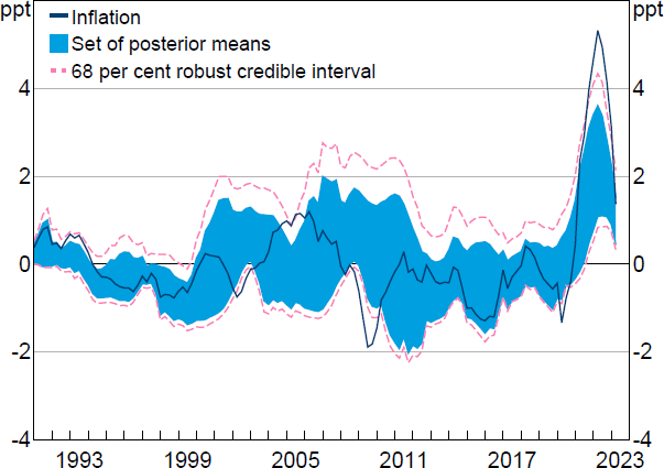
I assume a Jeffreys' prior over $\varphi ,{\pi }_{\varphi }\propto {\left|\Sigma \right|}^{-\left(n+1\right)/2}$, which is truncated to the region where the VAR is stable. This implies that the posterior for $\varphi$ is a (truncated) normal-inverse-Wishart distribution.^[34] Figure A1 presents the set of posterior means for the historical decomposition of year-ended growth in the GDP deflator alongside a 68 per cent robust credible interval. The set of posterior means for the supply contribution is somewhat wider on average than the set conditional on the OLS estimates of $\varphi$ (presented in Section 4.1).^[35] The robust credible intervals have excluded zero since late 2021, suggesting that, after accounting for statistical uncertainty, there is strong evidence that supply shocks have contributed positively to inflation outcomes in this period. To quantify this more precisely, I compute the posterior lower and upper probabilities that the contribution of the supply shock to year-ended inflation is positive; these are, respectively, the smallest and largest posterior probabilities assigned to the hypothesis that $H_{1,t}\ge 0$ obtainable within the robust Bayesian class of posteriors. In the March quarter 2022 (when inflation peaked), the posterior lower probability that the supply shock was contributing positively to inflation was 95 per cent and the posterior upper probability was 100 per cent.

Footnotes

Uncertainty around historical decompositions is often ignored. Notable exceptions are Antolín-Díaz and Rubio-Ramírez (2018) and Bergholt et al (2024). [31]

Granziera, Moon and Schorfheide (2018) develop a Bonferroni approach to construct asymptotically valid frequentist confidence sets for impulse responses or FEVDs in set-identified SVARs. They do not consider conducting inference about historical decompositions. [32]

Some papers specify the prior directly over the structural parameters (e.g. Baumeister and Hamilton 2015), but such a prior can also be represented as the product of a prior for $\varphi$ and a conditional prior for Q. Baumeister and Hamilton (2018) explain how to conduct Bayesian inference about historical decompositions and FEVDs under a single prior distribution. [33]

The VAR is stable in 84 per cent of draws from the (non-truncated) posterior. [34]

The two sets should coincide asymptotically. See Giacomini and Kitagawa (2021) for a discussion of the frequentist properties of their robust Bayesian procedure. [35]