RDP 2023-04: Can We Use High-frequency Yield Data to Better Understand the Effects of Monetary Policy and Its Communication? Yes and No! Appendix A: Affine Term Structure Model
May 2023
- Download the Paper 1.43MB
We use a simple nominal ATSM model to decompose yield changes.
In the model the one-period nominal interest rate rt is given by
where is a scalar and is a vector, so that rt is a linear function of the n pricing factors Xt. We assume that the data-generating process (also called the ‘real-world distribution’ or ‘P-dynamics’) of these pricing factors is a vector autoregressive process with one lag
where is an n×1 vector of intercepts, is an n×n matrix describing the evolution of Xt, and the n error terms .[16] Combining Equations (A1) and (A2) shows that the evolution of the short-term rate is controlled by the P-dynamics.
Following Duffee (2002), we assume that the market price of risk is also a linear function of the factors and is given by
where is an n×1 vector that represents the price of risk associated with each of the factors at time t, is an n×1 vector and is an n×n matrix. The specification implies that for each factor i, the compensation demanded by investors for bearing the risk associated with that factor is a constant plus a linear combination of all the factors.
If we impose a no arbitrage condition and assume a particular functional form for how agents price risk (stochastic discount factor), Equations (A1) to (A3) imply a set of pricing equations for zero-coupon nominal bond yields. In particular,
where is the yield at time t for an n-period zero-coupon nominal bond (i.e. a bond that matures in n periods), and An and Bn are functions of the underlying model parameters (see, for example, Hambur and Finlay (2018) for further details).
Of note, the bond pricing equations would be exactly the same if we took the true P-dynamics and allowed risks to be priced, and if we assumed investors were risk neutral (so ) but the pricing factors Xt followed some other risk-adjusted (or risk-neutral) dynamics, often referred to as the ‘Q-dynamics’
for and . In the literature and are often referred to as ‘P parameters’ as they determine the real world or P-dynamics, while and , or equivalently, and , are referred to as ‘Q parameters’.
Given observational equivalence of these two situations it can be difficult to estimate the coefficients. More formally, the likelihood surfaces tended to be ill-behaved (i.e. have multiple local minima and flat areas). To address this we take the approach of Adrian, Crump and Moench (2013) (ACM), who show that the parameters of an ATSM can be estimated using a simple three-step linear regression process. This helps to separate out the P- and Q-dynamics, similar to the Joslin, Singleton and Zhu (2011) (JSZ) normalisation.
A further complication in these models is a lack of information on the dynamics of short-term interest rates, given the short sample and high persistence of these rates. This makes it difficult to estimate the P-dynamics, and can bias down the estimated persistence of expected interest rate changes, therefore overstating the importance of changes in term premia (e.g Bauer, Rudebusch and Wu 2012). This reflects the well-known bias in regressions of highly persistent variables (e.g. Nicholls and Pope 1988).
We address this approach by incorporating surveys of expected short-term rates, in the vein of Kim and Orphanides (2012) and Guimarães (2016). This effectively gives us additional information about the dynamics of short-term rates by providing extra cross-sections.
In particular, we can think of the survey for the short rate in n periods being given by:
We take the surveys to be a noisy measure of the true expectation. As such, we shift to a maximum likelihood framework and include the likelihood of the survey data along with those of the pricing factors and the bond yields in the numerical optimisation.
KMS take a different approach, using statistical adjustments to overcome the persistence issue. We explore this approach using a bootstrap small-sample adjustment as in Malik and Meldrum (2016). However, doing so leads to a time series of expected interest rates that is less believable, compared to the survey model results (see below).
Consistent with ACM, our factors are the first K principal components from a panel of nominal interest rates. We use zero-coupon yields estimated using the methodology in Finlay and Olivan (2012), with maturities of n = 2,3,… and 120 months. We use four factors.
In calculating holding period returns – which are used in the ACM approach – we take the 1-month zero-coupon yield to be the short-term risk-free interest rate, and calculate returns for zero-coupon bonds with maturities of n = 6,12,18,24,36,… and 120 months. This gives us 12 cross-sectional units. The model is estimated at a monthly frequency.
We estimate the parameters of the model using data from mid-1992 to 2016. We end the sample in 2016 to avoid any potential issues introduced by rates nearing the effective lower bound. There may be some argument for excluding the early 1990s as inflation targeting was only introduced in this period, and so inflation dynamics could differ substantially. However, as argued by Guimarães (2016), inclusion of such a transition period can help substantially with identification of model parameters. That said, as long as surveys are included, excluding this early period from the sample doesn't change the ATSM estimates substantially.
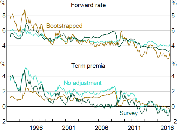
Figure A1 shows the results. Focusing on 5-year rates, we can see that the model with surveys shows a rise in expected rates through the mid-2000s, alongside strong economic outcomes and the early phase of the mining boom. Rates then fall around the GFC. In contrast, the bootstrapped model shows long-term expected rates decline over the mid-2000s, and spike during the GFC. Similar counterintuitive dynamics are evident for term premia, with the estimated term premia dropping sharply during the GFC in the bootstrapped model. Unsurprisingly, the expected rates are quite similar to those obtained in the joint term structure model estimated in Hambur and Finlay (2018), while the term premia follow a similar path to those in Kim and Orphanides (2012) for the United States.
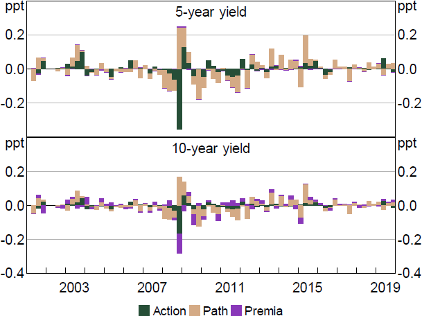
As discussed in the main text, using the ATSM model leads to somewhat different estimated Path and Premia shocks, and differing estimated macroeconomic effects. This is evident in Figure A2, which shows that Premia shocks seem to account for a much smaller share of the variation in yields when using the bootstrapped model. This is consistent with this model making expected rates substantially more flexible.

Note: Nominal ATSM with four factors.

Notes: Decomposition based on regression of yield changes on shocks. Residuals excluded. Quarterly sum.
Footnote
The relatively restrictive error assumption used here, and throughout the paper, is unlikely to hold in the data. While we could allow for more complex error structures, doing so would significant increase the complexity of the model. Moreover, Bikbov and Mueller (2011) find that doing so helps models match higher-order moments of the data, but not the first moments (i.e. yields). [16]