RDP 2023-03: Doing Less, with Less: Capital Misallocation, Investment and the Productivity Slowdown in Australia 6. Aggregate Implications
March 2023
- Download the Paper 1.26MB
The above results suggest that the relationship between capital growth and productivity has weakened, and that the flow of capital towards more productive firms has slowed. This is likely to have contributed to slower aggregate productivity and output growth as inputs are allocated less efficiently. But by how much?
To answer this, we use an approach similar to Andrews and Hansell (2021) and Hambur (forthcoming), and initially proposed in Decker et al (2020). The basic idea of the approach is to construct a counterfactual productivity index of what would have happened had the relationship between growth and productivity not weakened. In such a case, more productive firms would have been bigger, and so aggregate productivity would have been higher. We can compare the index to actual outcomes, to get a sense of the lost productivity and income.
More precisely, we create indices of aggregate labour productivity that combine actual realisations of firm-level MFP with input shares predicted from an estimated model.[19] The idea is that by varying the strength of the relationship between input growth and productivity, and therefore growth in inputs for different firms, we can construct counterfactual productivity indices that allow us to understand how aggregate productivity would have evolved had reallocation not slowed.
This approach is similar to the one taken in both Andrews and Hansell (2021) and Hambur (forthcoming). However, they focus solely on labour reallocation. Instead, we focus on both labour and capital. The advantage is that by using both inputs, alongside the estimated production functions, we can construct aggregate input indices for the firm, similar to Adelet McGowan, Andrews and Millot (2018). By combining these aggregate input indices with our MFP estimates we can consider what would have happed to aggregate income in the economy, not just labour productivity.
It is important to note that this approach isolates one, very direct channel through which slower reallocation of resources to high-productivity firms could have weighed on aggregate growth: through lower aggregate MFP. It abstracts from any effects slower reallocation of capital could have on the aggregate size of the capital stock, which, based on Figures 3 and 5, could be substantial. It also abstracts from any indirect effects the decline in dynamism could have on firm-level productivity, as examined in Andrews et al (2022).
We consider two different models: i) where the responsiveness of employment and capital growth to (lagged) productivity is allowed to decline; and ii) where the responsiveness is held constant at the level estimated at the start of the sample. These models give different predictions for employment and capital growth in time t+1. We can then combine these predictions with the (initial) level of employment and capital for the firm in t to get predicted inputs.
With these predictions in hand, we can construct three different productivity indices: one using observed input shares in the previous year (Equation (7)); one using the using the shares where the reallocation is allowed to vary (Equation (8)); and one using the share from the model where reallocation is held steady (Equation (9)). More formally:
The difference between the base index and either of the other indices shows the predicted productivity growth due to changes in the strength of reallocation. For example, the predicted gains in productivity based on the model with varying reallocation is:
The difference in these differences then captures how much slower aggregate productivity growth will be due to slower reallocation:
Given we are constructing a counterfactual for MFP, the results can also be thought of as a counterfactual for output growth, due to one-to-one relationship in simple production functions.[20]
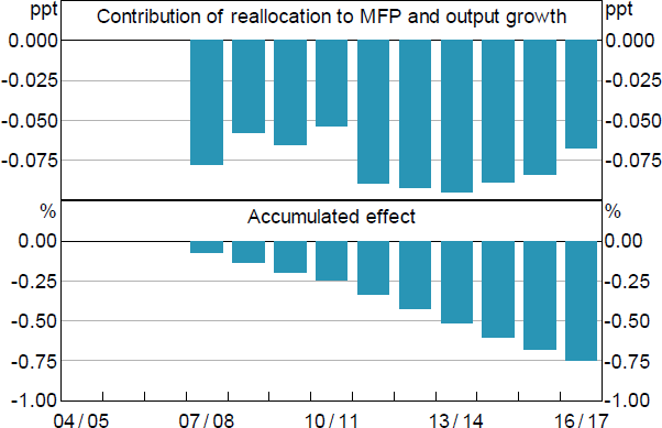
Figure 6 shows the results from this exercise. Looking through the volatility, if the relationship between growth and productivity had not weakened, and therefore more productive firms had tended to be larger, aggregate MFP and output growth would have been moderately stronger in each year since 2008. Accumulating this lost growth over the entire period, aggregate real output would have been around 0.75 per cent higher by 2017. This equates to output being around $13 billion lower than it would have been otherwise, and incomes being around $550 lower per capita or $1,000 per worker (in 2017 dollars).

Notes: Based on coefficient in Table 1, column 2. Excludes mining, agriculture and utilities.
To give some sense of how this fits in with the overall slowdown in productivity over this period, Andrews and Hansell (2021) found that slower labour reallocation lowered labour productivity growth by around 0.15 percentage points per year in the mid-2010s compared to the early 2000s. This equated to around a quarter of the overall slowdown in non-mining non-financial private sector labour productivity over the period.
The decline in labour productivity they identify could reflect two factors: slower aggregate MFP growth due to slower growth for high MFP firms, which we explore in this paper; and slower capital deepening, due to slower reallocation of labour to firms with abundant capital, which we do not. Our work suggests that about half the observed slowdown reflected lower MFP growth.
Overall then, these results suggest that had the relationships between firms' employment growth and productivity and capital growth and productivity not weakened, more productive firms would have been substantially larger. This would have meant that both aggregate productivity and income would have been moderately higher, compared with what actually occurred.