RDP 2023-01: The Effect of Credit Constraints on Housing Prices: (Further) Evidence from a Survey Experiment 5. Aggregate Results
January 2023
- Download the Paper 1.55MB
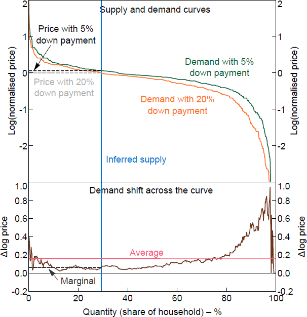
Comparing demand curves before and after the easing in collateral constraints reveals a clear pattern in the data (Figure 2). The upper end of the demand curve, with higher normalised WTPs, does not shift much while the lower end shifts substantially. The top panel of Figure 2 shows the demand curve constructed for each experimental down payment condition. Each demand curve shows the quantity demanded, on the horizontal axis, as a function of price on the vertical axis. The quantity is expressed as a share of total households in the sample because the raw number in the sample is not meaningful and there is no specific housing market that we are thinking about. The price is expressed relative to the home value, which allows the aggregation of WTPs from households who live in homes of different values, as outline in the method in Section 4. The figure shows the logarithm of the normalised price so shifts in demand can be interpreted as multiplicative changes (or approximate percentage changes). The lower panel shows just the shift in demand, which makes the pattern easier to see and highlights the difference between the average change and the change in the marginal buyer.
Table 1 shows my central estimates and bootstrapped confidence intervals for the change in the WTP of the marginal buyer (i.e. the price) assuming inelastic supply, and compares them to the average change in WTPs.[6] The WTP of the marginal buyer rises by around 6 per cent when collateral constraints are eased, which is significantly less than the 16 per cent average rise in WTPs. The pattern of the shift in demand curves and the difference between the average effect on WTPs and the effect on the marginal buyer are consistent with the idea that households who respond most to collateral constraints tend to have WTPs that are too low to affect the market price.

Note: The normalised price is relative to the home value given in the survey data.
Sources: Author's calculations; Fuster and Zafar (2021)
| Looser collateral constraint | Lower mortgage rate | Inherit US$100,000 | |
|---|---|---|---|
| Average WTP change | 0.16 (0.14–0.18) | 0.04 (0.04–0.05) | 0.11 (0.09–0.13) |
| Change in marginal WTP | 0.06 (0.04–0.08) | 0.05 (0.03–0.06) | 0.07 (0.06–0.10) |
| Difference | 0.10 (0.07–0.12) | 0.00 (–0.02–0.10) | 0.04 (0.03–0.07) |
|
Notes: Data are trimmed at 5 per cent based on (WTP) in each experiment, as in Fuster and Zafar (2021). Respondents with WTP equal to home value in either of the scenarios are excluded for each experiment (see Appendix B.3 for details). |
|||
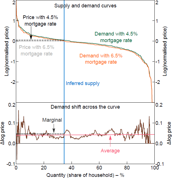
I compare the demand curves before and after the interest rate change using the same method. In this case, there is not much of a pattern across the demand curves with a higher interest rate compared to the demand curve with a lower interest rate (Figure 3). There is no systematic relationship between the change in WTP and the location on the demand curve, and consequently there is no difference between the change in the marginal buyer's WTP and the average change.
There was no debt-servicing restriction in the experimental questions, so changing the mortgage rate does not relax any hard constraints. As such there is no real reason to expect a systematic relationship between the shift of the demand curve across the market. Fuster and Zafar (2021) report that the interest rate effect is on the lower end of the range of empirical estimates, and that the uncertainties in how survey respondents interpret the effect on the term structure make the result a bit hard to benchmark. Further, if survey respondents are taking the interest rate cut as applying only to them, these results may miss an amplifying general equilibrium-type of effect that would operate through the home value (see Appendix A.1).

Note: The normalised price is relative to the home value given in the survey data.
Sources: Author's calculations; Fuster and Zafar (2021)
The average effect of the collateral constraint change is much larger than the average effect of the interest rate change, as reported in Fuster and Zafar (2021). But viewed through the lens of the marginal buyer method, the effects of the two changes have similar magnitudes.
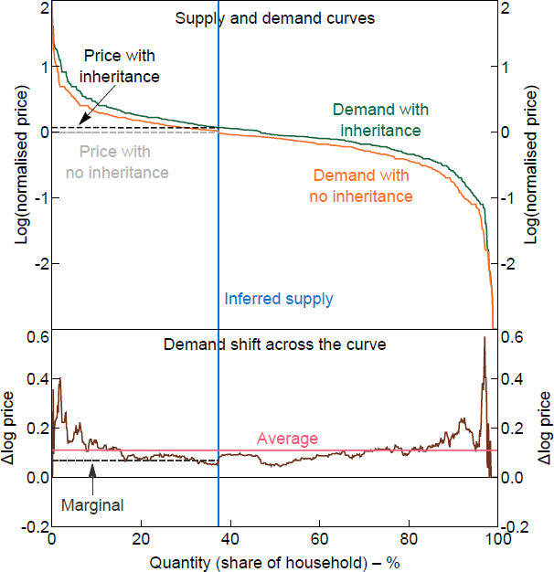
The demand curves for the inheritance experiment show more of a pattern than the mortgage rate experiment, but less than the down payment experiment (Figure 4). Constrained households are likely to have their constraints eased by the inheritance, which might suggest it should have the same structure as the down payment scenario. On the other hand, the inheritance can be used for anything – there is no guarantee a respondent would choose to put it toward a home.

Note: The normalised price is relative to the home value given in the survey data.
Sources: Author's calculations; Fuster and Zafar (2021)
Footnote
Appendix B.1 shows that the confidence intervals are similar for a range of different bootstrap methods as well as a non-parametric binomial method. [6]