RDP 2022-09: Estimating the Effects of Monetary Policy in Australia Using Sign-restricted Structural Vector Autoregressions 3. Estimates under Different Sets of Sign Restrictions
December 2022
- Download the Paper 1.84MB
This section presents estimates of impulse responses to a standard deviation monetary policy shock under different sets of identifying restrictions. Section 3.1 describes the specification of the reduced-form VAR. The subsequent sections describe the different sets of sign restrictions that are imposed and present the estimates obtained under each set of restrictions. I consider different sets of restrictions individually and in combination to disentangle their informativeness. Throughout, I report results based on the standard Bayesian approach to inference with a conditionally uniform prior for Q along with results based on the robust Bayesian approach to inference.
3.1 Specification of reduced-form VAR
The model includes a domestic block and a foreign block. The domestic block includes the interbank overnight cash rate (CASHt), real GDP (GDPt), trimmed mean CPI (CPIt) and the nominal trade-weighted exchange rate index (TWIt) defined such that higher values correspond to an appreciation of the Australian dollar. The foreign block of the model includes the terms of trade (TOTt), US real GDP (USGDPt) and the federal funds rate (FFRt).[8] The choice of variables is broadly consistent with previous SVAR analyses of the Australian economy, including Brischetto and Voss (1999), Dungey and Pagan (2000, 2009), Berkelmans (2005), Lawson and Rees (2008), Liu (2008), Jääskelä and Smith (2011), Jacobs and Rayner (2012) and Manalo, Perera and Rees (2014). All variables enter the model in log levels except for interest rates, which enter in levels. Consistent with Australia's status as a small open economy, the contemporaneous and lagged values of the foreign variables enter as exogenous variables in the equations for yt = (CASHt,GDPt,CPIt,TWIt)′. The model includes four lags of all variables and a constant. In the notation of Equation (1), zt is a vector containing (1,TOTt,USGDPt,FFRt)′ as well as four lags of the foreign variables.
The estimation sample begins in the March quarter 1984 (following the floating of Australia's exchange rate in December 1983) and ends in the December quarter 2019 (before the onset of the COVID-19 pandemic). The start of the sample period is similar to that in other SVAR analyses of the Australian economy, including Berklemans (2005) and Lawson and Rees (2008).
The prior for the reduced-form parameters is the non-informative Jeffreys prior, so The posterior is a normal-inverse-Wishart distribution, from which it is straightforward to obtain independent draws (e.g. Del Negro and Schorfheide 2011). All results are based on 1,000 draws from the posterior of such that the identified set is non-empty.
3.2 Sign restrictions on impulse responses
To begin, I impose the following set of sign restrictions on the impulse responses to a monetary policy shock.
Restriction (1): In response to a positive monetary policy shock at time t, the response of CASHt+h is non-negative and the response of CPIt+h is non-positive for h = 0,1,2,3.
These restrictions impose that the cash rate does not decrease and the CPI does not increase in the year after a positive monetary policy shock. The pattern of restrictions is, in principle, the minimum required to differentiate monetary policy shocks from shocks to supply and demand; conventional theory suggests that a positive monetary policy shock should raise the interest rate and lower prices, while both supply and demand shocks should move the interest rate and prices in the same direction. The restrictions are similar to those considered in Uhlig (2005), who estimates the effects of US monetary policy.[9] Note that the responses of output and the exchange rate are left unrestricted. The horizon over which the impulse responses are restricted is somewhat arbitrary. Uhlig explores different choices of horizon up to a maximum of two years. My choice reflects a belief that monetary policy shocks are likely to have moderately persistent effects. I am hesitant to impose restrictions at horizons much longer than one year, since these restrictions become less credible as the horizon increases, and I want to consider restrictions that are likely to be uncontroversial.[10]
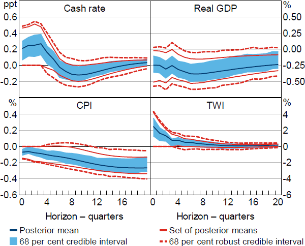
Figure 1 plots impulse responses to a positive, standard deviation monetary policy shock obtained under Restriction (1). When using the standard Bayesian approach to inference, and based on the posterior mean, the shock results in the cash rate increasing by about 20 basis points on impact. Output responds sluggishly and is about 0.2 per cent lower at the two-year horizon. There is a reasonably high posterior probability (around 80 per cent) that the output response is negative at this horizon. Prices also decline persistently and the real exchange rate appreciates on impact before depreciating. Overall, these results are broadly consistent with conventional macroeconomic theory, although they are subject to considerable uncertainty; the 68 per cent credible intervals include zero at most horizons.[11]
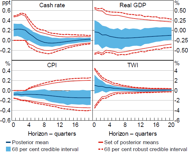
Notes: Restrictions on impulse responses of the cash rate and CPI. Impulse responses are to a positive, standard deviation monetary policy shock.
To what extent are these results sensitive to the choice of conditional prior? To answer this question, I plot the set of posterior means and 68 per cent robust credible intervals obtained using the robust Bayesian approach to inference. Focusing on the output response, the set of posterior means contains zero at all horizons and the posterior lower probability (the smallest posterior probability over the class of posteriors) that the output response is negative after two years is zero. This implies that there are conditional priors that are consistent with the identifying restrictions and that yield posteriors assigning probability one to the hypothesis that output increases two years after the shock. The set of posterior means for the response of prices also includes fairly large positive responses at horizons beyond one year (i.e. beyond the horizons that are restricted to be non-positive), so the data and identifying restrictions cannot rule out the presence of price puzzles. The set of posterior means for the exchange rate response includes large negative responses on impact; this is at odds with ‘exchange rate overshooting’, which is a prediction of conventional open economy models (Dornbusch 1976). Overall, posterior inferences under the standard Bayesian approach appear to be largely driven by the choice of conditional prior. After eliminating this source of posterior sensitivity, the identifying restrictions cannot rule out responses that are at odds with conventional macroeconomic theory, and the identifying restrictions appear to be fairly uninformative about the effects of monetary policy.
Wolf (2020) explains that the apparent expansionary effects of monetary policy shocks obtained under standard sign restrictions on impulse responses may reflect linear combinations of demand and supply shocks ‘masquerading’ as monetary policy shocks. The intuition is that a linear combination of expansionary demand and supply shocks can result in the nominal interest rate increasing and prices decreasing. Because these responses satisfy the sign restrictions used to identify the monetary policy shock, the identified sets for the impulse responses obtained under the sign restrictions are contaminated by linear combinations of impulse responses to these expansionary demand and supply shocks. This suggests that it is necessary to impose additional identifying restrictions to better disentangle the monetary policy shock from other shocks.
To this end, I consider imposing additional restrictions. As noted above, the set of posterior means for the response of the exchange rate obtained under Restriction (1) includes negative responses, which is at odds with conventional macroeconomic theory; standard models imply that the exchange rate should appreciate on impact in response to a positive monetary policy shock before depreciating. This motivates the following set of restrictions, which augments Restriction (1) with a restriction on the response of the exchange rate.
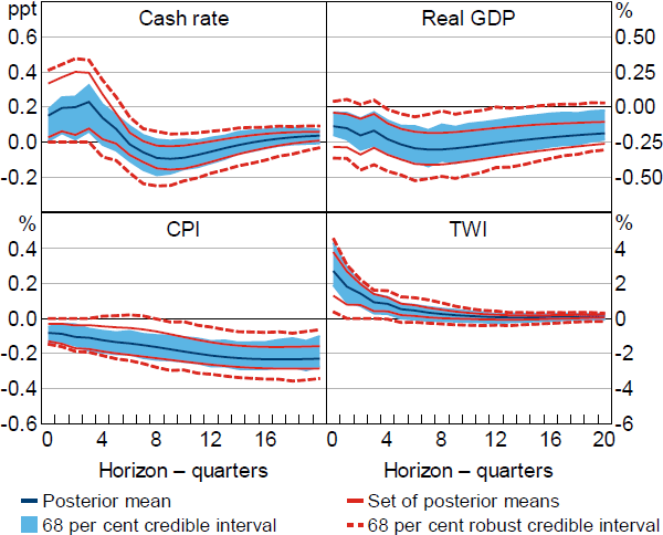
Restriction (2): In response to a positive monetary policy shock at time t, the responses of CASHt+h and TWIt+h are non-negative and the response of CPIt+h is non-positive for h = 0,1,2,3.
As seen in Figure 2, the results under these additional restrictions are little changed from those under Restriction (1) (with the obvious exception of the response of the exchange rate, whose response is restricted). The restrictions on the response of the exchange rate therefore do not appear to mitigate the problem of masquerading shocks.
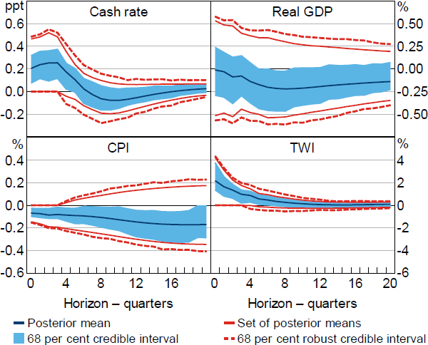
Notes: Restrictions on the impulse responses of the cash rate, CPI and TWI. Impulse responses are to a positive, standard deviation monetary policy shock.
3.3 Sign restrictions on the monetary policy reaction function
As an alternative to imposing further restrictions on impulse responses, I follow Arias et al (2019) and consider restricting the structural coefficients in the equation for the cash rate, which can be interpreted as the monetary policy reaction function. For instance, the coefficients on prices and output are restricted so that monetary policy is not loosened in response to higher output or prices.[12] These restrictions are consistent with monetary policy rules that are typically embedded in macroeconomic models. Moreover, Wolf (2020) explains that these restrictions can help mitigate the masquerading shocks problem. Using a simple New Keynesian model as a data-generating process, he shows that the misidentification of linear combinations of expansionary supply and demand shocks as monetary policy shocks means that the identified structural equation for the nominal interest rate is actually a linear combination of the IS curve, Phillips curve and Taylor rule. When the weight assigned to the true monetary policy shock is small, the implied coefficient on output in the misidentified Taylor rule has the wrong sign. Restricting the sign of this coefficient largely removes the effect of the masquerading supply and demand shocks by ruling out identified shocks that assign small weight to the true monetary policy shock.
To be more concrete, consider the first equation in the SVAR, which I interpret as the monetary policy reaction function:
where is the (1, i) th element of A0. The sign normalisation implies that Consequently, the reactions of the cash rate to output and prices are non-negative if and .
I initially replace the restrictions on impulse responses with restrictions on the coefficients in the reaction function and later combine the two sets of restrictions. This allows me to isolate the informativeness of the restrictions on the reaction function. I maintain the restriction that the cash rate responds positively to the monetary policy shock, so I am always identifying impulse responses to a shock that raises the cash rate on impact.
Restriction (3): The coefficients on GDPt and CPIt in the structural equation for CASHt, a12 and a13, are non-positive, and the impact response of CASHt to the monetary policy shock is non-negative.
Under Restriction (3) and using the standard approach to Bayesian inference, the output response is negative with high posterior probability (Figure 3); the posterior mean indicates that output falls by about 0.3 per cent on impact and remains around this level for two to three years, and the posterior probability of a negative output response after two years is close to 95 per cent. There is reasonably strong evidence that prices – whose response is unrestricted under this set of restrictions – decline with some delay; the posterior probability that the price response is negative is a bit over 80 per cent at the two-year horizon. The credible intervals for the response of the TWI include zero at all horizons. Overall, the results obtained under the conditionally uniform prior suggest that the restrictions are quite informative about the effects of monetary policy on output and prices. However, as in the case where the sign restrictions were imposed on the impulse responses, the results are sensitive to the choice of conditional prior; the set of posterior means includes zero for all variables and horizons.
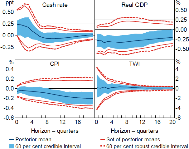
Notes: Restrictions on coefficients in the monetary policy reaction function (real GDP and CPI). Impulse responses are to a positive, standard deviation monetary policy shock.
The coefficient on the exchange rate was left unrestricted under Restriction (3). However, it seems plausible that the central bank may take into account the exchange rate when setting policy, including indirectly via its effects on forecasts of other macroeconomic variables.[13] For example, an appreciation of the exchange rate will put downward pressure on consumer prices due to the direct effect of lower import prices. It will also lead to a decline in exports, which will weigh on output. To the extent that these developments occur with a lag and the central bank sets policy in a forward-looking manner, it may therefore want to cut the policy rate in response to the appreciation. This motivates restricting the coefficient on the exchange rate. The set of posterior means for the coefficient on the exchange rate under Restriction (3) is [–0.25,0.24], so restricting this coefficient to be non-negative will truncate (at least at some values of ) and thus may result in more informative inference about the impulse responses.[14] I therefore consider the following set of restrictions, which extends the restrictions on the systematic component of monetary policy introduced in Arias et al (2019) to the open economy setting.[15]
Restriction (4): The coefficients on GDPt and CPIt in the structural equation for CASHt, a12 and a13, are non-positive, the coefficient on TWIt, a14, is non-negative, and the impact response of CASHt to the monetary policy shock is non-negative.
Relative to Restriction (3), the additional restriction on the exchange rate coefficient leads to more informative inference about the output response; the set of posterior means for the output response excludes zero at horizons beyond one year and the output response is negative at the two-year horizon with a posterior lower probability of around 75 per cent (Figure 4). The estimates do not rule out increases in prices at short-to-medium horizons, although prices fall with high posterior lower probability at longer horizons. The restriction reduces the prominence of negative exchange rate responses, although the posterior lower probability that the exchange rate appreciates on impact is still only around 25 per cent.
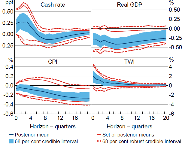
Notes: Restrictions on coefficients in the monetary policy reaction function (real GDP, CPI and TWI). Impulse responses are to a positive, standard deviation monetary policy shock.
Overall, comparing the results in Figures 2 and 4, it appears that restrictions on the monetary policy reaction function are more informative about the responses of output and prices to a monetary policy shock than restrictions on the impulse responses. However, the restrictions do not rule out positive price responses at short-to-medium horizons or an exchange rate depreciation on impact. Both of these results are at odds with conventional macroeconomic theory.
3.4 Combining sign restrictions on impulse responses and reaction function
Given the inability of restrictions on the monetary policy reaction function to rule out price puzzles and exchange rate depreciations, I consider combining these restrictions with restrictions on the impulse responses. For this exercise, I include the restrictions relating to the exchange rate.
Restriction (5): In response to a positive monetary policy shock at time t, the responses of CASHt+h and TWIt+h are non-negative and the response of CPIt+h is non-positive for h = 0,1,2,3. Additionally, the coefficients on GDPt and CPIt in the structural equation for CASHt, a12 and a13, are non-positive and the coefficient on TWIt, a14, is non-negative.
Under Restriction (5), output falls with high posterior lower probability at horizons between one and three years (Figure 5). For example, the posterior lower probability of a negative output response at the two-year horizon is about 95 per cent. Combining the restrictions reduces the prominence of price puzzles at short-to-medium horizons, although a positive price response is not ruled out entirely; for instance, the posterior upper probability of a positive price response at the two-year horizon is about 40 per cent. Prices fall with high posterior lower probability at longer horizons; the posterior lower probability of a negative price response is at least 90 per cent at horizons greater than three years. Overall, the restrictions appear to be reasonably informative about the effects of monetary policy when combined, in the sense that output, prices and the TWI all respond to monetary policy in a way that is consistent with macroeconomic theory with high posterior probability regardless of the choice of conditional prior, at least at longer horizons.
Notes: Restrictions on impulse responses (cash rate, CPI and TWI) and coefficients in the monetary policy reaction function (real GDP, CPI and TWI). Impulse responses are to a positive, standard deviation monetary policy shock.
3.5 Restrictions on relationship with a proxy variable
Although Restriction (5) appears to be fairly informative about the macroeconomic effects of monetary policy shocks, additional credible restrictions could be valuable in reducing uncertainty. One possible approach is to impose restrictions on the impulse responses to other shocks or on the coefficients in other structural equations. However, this requires making assumptions about the nature of these other shocks or equations; for example, based on predictions from a macroeconomic model (e.g. Jääskelä and Jennings 2010). Instead, I consider alternative restrictions that are not tied to a particular macroeconomic model.
Specifically, I impose restrictions on the relationship between the monetary policy shock and an existing proxy for that shock. The proxy is taken from Beckers (2020), who applies a variant of the approach in Romer and Romer (2004) to purge the cash rate of its endogenous response to economic conditions. He additionally controls for the systematic response of the cash rate to credit conditions (measured by money market spreads) and uses cash rate expectations (proxied for by estimated zero-coupon forward rates) to further purge the cash rate of variation that is anticipated by financial market participants. I use this ‘unanticipated’ change in the cash rate as a proxy for the monetary policy shock.
The proxy in Beckers (2020) was constructed with the purpose of measuring monetary policy shocks, so it is natural to assume that the proxy is positively correlated with the monetary policy shock. Additionally assuming that the proxy is contemporaneously uncorrelated with all other structural shocks (i.e. exogenous) implies that the proxy can be used to point identify the monetary policy shock in a proxy SVAR (e.g. Stock and Watson 2018).[16] However, even though this measure is purged of many potentially endogenous drivers of the cash rate, the exogeneity condition is still quite strong and will be violated if the variables used to purge the cash rate of its endogenous response to economic and financial conditions do not control for the RBA's response to all other shocks hitting the economy.
To relax this assumption, I instead impose restrictions that the proxy and the true monetary policy shock are positively correlated, and that variation in the proxy primarily reflects the monetary policy shock.[17] This allows me to incorporate the information included in the proxy while allowing the proxy to be contaminated by other shocks. Because I do not impose exogeneity with respect to nonmonetary policy shocks, the impulse responses remain set identified and I can continue to impose the other sign restrictions considered above.
More formally, assume that the proxy, mt, contains information about the structural shocks according to the process
where independently of . Substituting out using the SVAR representation yields the ‘first-stage regression’ of the proxy on the contemporaneous and lagged values of the variables entering the VAR:
where and are reduced-form parameters that are identified from the regression of mt on yt and xt. The covariance between the proxy and the structural shocks is
Restrictions on elements of can therefore be expressed as restrictions on Q, where the restrictions are a function of the reduced-form parameters in the VAR for yt and the first-stage regression. The restriction that mt is positively correlated with the monetary policy shock, , is equivalent to , which is a linear inequality restriction on the first column of Q .[18] The contribution of the i th structural shock to the variance of mt is
If the contribution of the monetary policy shock to the variance of the proxy is greater than that of any other shock, then This is equivalent to the restriction that the correlation between mt and the monetary policy shock is greater in absolute value than the correlation between mt and any other structural shock, Given that the correlation between the proxy and the monetary policy shock is positive, this is equivalent to
which can be expressed as a system of linear inequalities in vec(Q).
The vector of reduced-form parameters is now augmented with the parameters from the reduced-form process for the proxies, so . Following Giacomini et al (2022b), I assume a (non-informative) Jeffreys prior for the reduced-form parameters in the first-stage regression that is independent of the prior over the reduced-form VAR parameters. The proxy from Beckers (2020) is available from the March quarter 1994 to the December quarter 2018. I continue to estimate the VAR over the same (longer) sample used above, and use the sample over which the proxy is available to estimate the first-stage regression.
I augment the restrictions on impulse responses and the monetary policy reaction function with the proxy-based restrictions.
Restriction (6): In addition to the restrictions in Restriction (5), mt is positively correlated with the monetary policy shock and the contribution of the monetary policy shock to the variance of the proxy is greater than the contribution of any other structural shock.
The set of posterior means for the correlation between the proxy and the monetary policy shock, , is [0.14, 0.22] and the 95 per cent robust credible interval is [0.05, 0.40]. This suggests that the proxy and monetary policy shock are fairly weakly correlated. Nevertheless, the additional restrictions appear to sharpen identification relative to Restriction (5); for example, as seen in Figure 6, the set of posterior means for the output response at the two-year horizon obtained under Restriction (6) is about 60 per cent as wide as the set obtained under Restriction (5). A natural question is whether the apparent informativeness of the proxy is because the VAR does not span the relevant information set. For instance, credit spreads are used to construct the proxy but are not included in the VAR. Section 5.3 presents estimates from a model that includes credit spreads.[19]
Notes: Restrictions on impulse responses (cash rate, CPI and TWI), coefficients in the monetary policy reaction function (real GDP, CPI and TWI), and relationship between monetary policy shock and proxy for the shock. Impulse responses are to a positive, standard deviation monetary policy shock.
The set of posterior means for the output response obtained under Restriction (6) excludes zero at all horizons, and the robust credible intervals exclude zero at horizons between one and four years. The additional restrictions also appear to largely rule out the price puzzle; the posterior lower probability that prices fall following the shock is greater than 80 per cent at all horizons and greater than 90 per cent at horizons longer than three years. Overall, the proxy variable appears to contain useful identifying information even when discarding the usual fairly strong exogeneity assumption and despite the proxy appearing to be only weakly correlated with the monetary policy shock.
3.6 Plausibility and informativeness of restrictions
This section quantitatively assesses the ‘plausibility’ of the restrictions, which is the degree to which the identifying restrictions are compatible with the observed data. It also systematically compares the informativeness of the different restrictions. The approaches to quantifying these concepts follow Giacomini and Kitagawa (2021).
3.6.1 Posterior plausibility
When there are a sufficient number of sign restrictions, the identified set may be empty at particular values of . The posterior probability that the identified set is non-empty – the ‘posterior plausibility’ – can be used to quantify the degree to which the identifying restrictions are consistent with the observed data (as summarised by the reduced-form parameters). If the posterior plausibility is zero (which will occur if every draw of yields an empty identified set), the identifying restrictions are inconsistent with the observed data. Conversely, if the identifying restrictions are correct, the posterior plausibility should approach one asymptotically as the sample size grows and the reduced-form posterior converges towards the true value of .
Under Restrictions (1)–(4), the posterior plausibility of the restrictions is one (i.e. the identified set is never empty), and it is greater than 99 per cent under Restriction (5). These restrictions therefore appear to be ‘plausible’ in the sense that they are consistent with the observed data. In contrast, the posterior plausibility of Restriction (6) is only around 45 per cent. However, as discussed in Giacomini, Kitagawa and Read (2022a), this does not necessarily mean that the restrictions are likely to be incorrect. In a finite sample, the posterior may assign probability to regions of the reduced-form parameter space that are ‘far’ from the true value, in which case the posterior plausibility may be low even when the identifying restrictions are correct.
3.6.2 Informativeness of restrictions
The informativeness of a given set of identifying restrictions can be quantified by comparing the width of the set of posterior means against that obtained under a less-restrictive model. Specifically, I compare the width of the set of posterior means of the output response at the two-year horizon under each set of restrictions against that obtained when the only restriction is that the impact response of the cash rate is non-negative (Table 1).[20] If the restrictions were point identifying, the informativeness measure would be 100 per cent.
| Restriction | |||||
|---|---|---|---|---|---|
| (1) | (2) | (3) | (4) | (5) | (6) |
| 13.1 | 17.7 | 25.9 | 54.5 | 64.3 | 78.2 |
| Note: Informativeness is measured as the percentage by which the set of posterior means for the output response at the two-year horizon narrows relative to a model where only the impact response of the cash rate is restricted; higher numbers indicate more-informative restrictions. | |||||
Based on this measure, the restrictions on the monetary policy reaction function are substantially more informative than the restrictions on the impulse responses; for instance, relative to the ‘unrestricted’ model, Restriction (1) shrinks the set of posterior means by 13 per cent, whereas Restriction (3) shrinks the set of posterior means by 26 per cent. Restriction (4), which adds a restriction on the systematic response to the exchange rate, shrinks the set of posterior means by over 50 per cent. The full set of restrictions (Restriction (6)) shrinks the set of posterior means by close to 80 per cent.
In principle, differences in the apparent informativeness of the identifying restrictions can arise from two sources: 1) differences in the extent to which the restrictions truncate the identified set on average over the reduced-form posterior; and 2) differences in the space of reduced-form parameters that have a non-empty identified set. Because the posterior plausibility is close to one for Restrictions (1)–(5), differences in the informativeness measure across these restrictions arise from the restrictions truncating the identified set to a greater or lesser degree. In contrast, because the posterior plausibility of Restriction (6) is around 45 per cent, the results under this set of restrictions are based on a different posterior distribution of reduced-form parameters. This makes it more complicated to directly compare the informativeness of Restriction (6) to the other sets of restrictions. To make a like-for-like comparison, I take the draws of the reduced-form parameters obtained under Restriction (6) and impose Restriction (5). Doing this returns results that are very similar to those obtained under Restriction (5), which suggests that it is the ability of Restriction (6) to truncate the identified set, rather than the different reduced-form posterior, which is driving the measured informativeness.[21]
Footnotes
Over the period following the global financial crisis, the federal funds rate was constrained by the zero lower bound and unconventional monetary policy was used to deliver stimulus to the US economy. The federal funds rate was therefore an imperfect indicator of the stance of US monetary policy during this period. I obtain similar results if I instead splice the federal funds rate with the ‘shadow federal funds rate’ constructed by Wu and Xia (2016), which is the predicted short rate from a model of the term structure of interest rates that does not feature a lower bound. [8]
Uhlig (2005) imposes additional restrictions that are designed to disentangle monetary policy shocks from shocks to money demand. Since my SVAR does not include any monetary aggregates, I do not consider such restrictions. Kim and Lim (2018) impose similar restrictions in models of several small open economies, including Australia. [9]
The results are similar when imposing the restrictions on impact only. [10]
The credible intervals presented under the standard Bayesian approach to inference are highest posterior density intervals, which are the shortest intervals that cover 68 per cent of the posterior. [11]
Arias et al (2019) note that central banks do not have access to contemporaneous data on output and prices when setting the policy rate. However, they typically have access to rich data that allows them to accurately nowcast these variables. Rather than modelling the process of information acquisition and nowcasting, their approach makes the simplifying assumption that the central bank has access to data on current output and prices when setting policy. They also impose zero restrictions on the coefficients of some monetary aggregates in the monetary policy reaction function, but such variables are not included in my model. [12]
The RBA's multi-sector model of the Australian economy includes the change in the real exchange rate in the Taylor rule (Gibbs et al 2018). The posterior mean of the coefficient on this variable is negative, but close to zero. [13]
The coefficient on the exchange rate (a14) does not represent the change in the cash rate in response to a 1 per cent appreciation, because the coefficient on CASHt (a11) is not normalised to equal one. The change in the cash rate in response to a 1 per cent appreciation (holding all else equal) would be −a14/a11. [14]
Castelnuovo, Pellegrino and Ranzato (2022) also consider imposing this restriction in the US context. They justify the restriction on the basis of narrative evidence. [15]
To estimate the effects of monetary policy shocks in Australia, Beckers (2020) includes the (cumulated) purged measure of the cash rate in an SVAR and imposes additional zero restrictions on the structural parameters (i.e. he does not use a proxy SVAR). [16]
These restrictions are also considered in Braun and Brüggemann (forthcoming). In a similar vein, Ludvigson, Ma and Ng (2017), Piffer and Podstawski (2018), Arias, Rubio-Ramírez and Waggoner (2021), Caggiano and Castelnuovo (2021) and Giacomini, Kitagawa and Read (2022b) impose sign restrictions on the correlations between structural shocks and variables that are external to the VAR. [17]
I write this restriction in terms of the covariance, but it is equivalent to a restriction on the correlation; to write the restriction in terms of the correlation, divide by . [18]
More generally, the fact that the VAR excludes information to which monetary policy responds (in particular, information summarised by the RBA's forecasts) means that the ‘true’ monetary policy shock may not be invertible (i.e. not recoverable as a linear combination of the reduced-form VAR innovations). However, if the true monetary policy shock is ‘close to’ invertible, it may still be possible to accurately identify the effects of the shock (Wolf 2020). It would be interesting to explore how misspecification of the reaction function in the SVAR affects identification when an externally generated proxy is available from an estimated reaction function that is plausibly (close to) correctly specified. [19]
The measured informativeness of the restrictions is similar when averaging over horizons. [20]
Approximation errors associated with the algorithm used to check if the identified set is non-empty mean that the posterior plausibility of Restriction (6) may be understated. Similarly, numerical approximation errors mean that the informativeness of Restriction (6) may be under or overstated. I attempt to minimise both problems by using a large number of draws of Q in the numerical approximation algorithms. See Appendix A for further details. [21]