Research Discussion Paper – RDP 2019-07 MARTIN Has Its Place: A Macroeconometric Model of the Australian Economy
August 2019
1. Introduction
This paper presents a model of the Australian economy. The model, called MAcroeconomic Relationships for Targeting INflation (MARTIN), is a macroeconometric model built to capture the key economic relationships relevant for the conduct of monetary policy in Australia. It consists of a series of estimated equations that closely match the forecasting approach used at the Reserve Bank of Australia (RBA). RBA staff use the model to interpret recent economic developments, analyse the implications of alternative risks and scenarios and generate forecasts of the economy's likely future evolution.
The impetus for developing MARTIN came from an external review of the RBA's forecasting tools and procedures (Pagan and Wilcox 2016). The review recommended expanding the RBA's analytical toolkit to include an economy-wide model that could draw together the vast array of single-equation forecasting models that RBA staff maintain. The aim was to build a model that would closely correspond to the way analysts and policymakers at the RBA think about how the economy evolves. This objective drove the development of MARTIN, from its modelling framework, scope, choice of variables and causal mechanisms.
MARTIN captures many features of the Australian economy and monetary policy transmission mechanism. Most equations are modelled in an error correction framework, which allows us to impose a theoretically coherent structure on the long-run properties of the model while retaining the flexibility to account for the short-run empirical relationships observed in the data. The key elements of the model are the expenditure components of GDP, the labour market, the determinants of inflation and some financial market variables. The key mechanisms in the model trace through the relationships between these variables. The level of economic activity depends on decisions by domestic firms and households, along with international trade. Households' decisions are influenced by their income and balance sheet position, business investment is largely demand-determined and trade flows depend on Australian and overseas demand as well as relative prices. Economic activity affects the demand for labour and so the degree of spare capacity in the labour market. Labour market spare capacity affects inflation directly as well as through its effect on wages which, along with other input costs, also influence prices.
Cusbert and Kendall (2018) explain the rationale and goals of MARTIN, and provide an outline of the model's structure. This paper covers some of the same ground, but includes a more detailed treatment of MARTIN's individual equations, as well as an illustration of the model's dynamic properties. The paper is structured as follows. Section 2 describes the principles underpinning the modelling framework and how it fits in to the RBA's approach to analysing economic developments. Section 3 provides an overview of the model. And Section 4 delves into MARTIN's equations. Readers who wish to avoid the technical details of the model may safely skip these two sections. Section 5 describes some of the key dynamic properties of the model and Section 6 concludes.
2. What is MARTIN and What is it Used for?
MARTIN is a macroeconometric model of the Australian economy. It describes relationships between key macroeconomic variables and is used to generate economic forecasts and conduct counterfactual scenario analysis. When developing the model, we had to make choices about what variables the model would capture, as well as its structure and estimation framework. A key objective in making these choices was to be consistent with the RBA's existing analytical and forecasting approach. This meant that we could easily integrate MARTIN into the RBA's processes and ensured that the model would be well understood by staff and policymakers. As such, while the model is large, its design is relatively simple and was developed in close consultation with the forecasting staff who are the main consumers of the model's output.
2.1 Model Variables
MARTIN aims to capture the mechanisms that matter most for a central bank; namely the features of the Australian economy that affect the setting and transmission of monetary policy. As such, the model centres on the interactions between the expenditure components of GDP (such as consumption and investment), prices and the labour market. Several components of the household balance sheet are modelled, as well as some financial market variables (such as the exchange rate and equity prices). MARTIN also includes exogenous variables that summarise overseas economic conditions.
Although the model is large and its equations capture numerous economic interactions, it does not cover every aspect of the economy. Like all models, MARTIN provides a simplified representation of reality. In order to remain tractable, it omits some variables that, in certain circumstances, could have a material influence on economic outcomes. Some notable omissions include a standalone banking sector, a detailed treatment of firms' income and balance sheets, industry detail and measures of economic agents' confidence or sentiment. Some features that are present in a limited way include the foreign and government sectors, productivity growth and other aspects of the supply side of the economy, expectation formation and stock-flow dynamics. Over time, we expect that further development of these aspects of the model will occur. Some of these extensions will be incorporated into the core of MARTIN, while others are likely to exist as satellite models that can be used in conjunction with MARTIN to address specific questions.
2.2 Model Framework
MARTIN is an economy-wide model. These types of models examine many economic variables at the same time, with only a few variables taken as given. That is, most variables in MARTIN are endogenous. MARTIN determines the value of its endogenous variables jointly as a system. Examining variables in a system is desirable for a number of reasons. As outlined in Atkin and La Cava (2017), monetary policy influences economic activity through multiple channels, such as through its effect on the housing market and the exchange rate. Examining variables in a system allows us to isolate the roles that individual channels play in determining aggregate economic outcomes, and aids our understanding of how monetary policy works. Economy-wide models also account for feedback between economic variables. For example, an increase in aggregate demand will encourage firms to hire more workers, which raises employment and lowers the unemployment rate. The tightening of the labour market is likely to lead to an increase in wages growth. The resulting increase in household incomes is likely to lead to an increase in consumption, further raising aggregate demand. Accounting for feedback mechanisms is particularly important for understanding medium- and longer-term developments, because over these horizons interrelationships between economic variables become more important and there are fewer leading indicators available.
A key feature of MARTIN is that many of its equations are based on the many single-equation models that the RBA already maintains.[1] However, differences between the equations in MARTIN and the single-equation models exist. For example, we have restricted the value of some coefficients in several of MARTIN's equations to ensure that the model has stable long-run properties. MARTIN's equations are also relatively parsimonious to ensure less volatile short-run model dynamics.
The RBA also maintains another economy-wide model: the multi-sector dynamic stochastic general equilibrium (DSGE) model, MSM, documented in Rees, Smith and Hall (2016) and extended by Gibbs, Hambur and Nodari (2018). This model is built on a consistent theoretical framework of optimising households and firms. The framework provides a clear interpretation of the causal mechanisms within the model, maintains internal consistency and has an explicit role for forward-looking expectations. This makes it useful for scenario analysis. However, in common with other DSGE models, MSM does not forecast as well as some other models, and its causal mechanisms do not always correspond to how policymakers think the economy works.[2] MSM also lacks some of the detail – particularly around the labour market and household balance sheets – that economists at the RBA use to analyse the economy, and it is difficult to modify to incorporate new variables or changing economic dynamics.
MARTIN lies between the two extremes of a fully data-driven model and one guided solely by theory.[3] Most of the model's estimated equations are error correction models (ECMs).[4] This methodology explicitly distinguishes between short-term dynamics and long-term equilibrium relationships. In MARTIN, economic theory influences the choice of what variables to include in each equation and, in some cases, how those variables relate to each other. This is particularly true for the long-run relationships in the model. But MARTIN is also designed to capture observed relationships in the data, particularly in its short-run dynamics. As such, most equations are estimated, although some relationships are calibrated to better fit our beliefs or external estimates. The benefit of this empirical approach is that MARTIN's equations are flexible enough to incorporate the economic mechanisms that policymakers at the RBA believe are important and yet still fit the observable relationships in the data reasonably well. The flexibility allows us to introduce features that are specific to the Australian economy, which can be difficult to incorporate in a DSGE model. This flexibility reflects the fact that the model is not derived from a single theoretical framework. The downside is that the causal mechanisms in MARTIN are less clear than in, say, a DSGE model.
So, although MARTIN might capture empirical relationships that exist in the data, the drivers of these relationships might in some cases be hard to interpret.
The development of MARTIN has coincided with an active debate about the merits of alternative approaches to building models for economic policy analysis. Blanchard (2018) and Wren-Lewis (2018) describe the benefits of macroeconometric models like MARTIN, with their flexibility and ability to match the data being key. Lindé (2018) offers a more sceptical appraisal. Although DSGE models remain widely used, several other central banks maintain macroeconometric models that are similar to MARTIN. Leading examples include the Federal Reserve's FRB/US model, the Bank of Canada's LENS model and the Bank of Japan's Q-JEM model (Brayton, Laubach and Reifschneider 2014; Gervais and Gosselin 2014; Fukunaga et al 2011). MARTIN is also similar in style to some previous models of the Australian economy, including AUS-M (Downes, Hanslow and Tulip 2014) and its predecessor, TRYM, which was developed by the Australian Treasury (Taplin et al 1993).[5]
2.3 Model Uses
RBA staff use MARTIN for four main tasks:
- enhancing the staff's understanding of recent economic developments and how their forecasts fit together;
- extending staff forecasts beyond the usual two-to-three year forecast horizon to generate medium- and long-run projections;
- generating model forecasts, for comparison to staff forecasts;
- producing scenarios to quantify uncertainties around the central forecasts.
We can use MARTIN to replicate the RBA staff forecasts (that is, the forecasts produced using single-equation models, real-time data and a range of off-model information, such as insights from liaison with businesses and other organisations) by appending ‘add factors’ to the equations. These ‘add factors’ are additional reduced-form errors that account for the differences between the staff and MARTIN forecasts. They reflect aspects of the forecasts that MARTIN cannot explain, and can be loosely considered as a proxy for the ‘judgement’ that the staff apply in producing their forecasts. While the existence of ‘judgement’ does not make the staff forecasts wrong, MARTIN's decompositions help the staff to gauge whether the judgements being made are appropriate, and whether they have been applied consistently across the forecasts. An example of where judgement may appear is if the staff forecasts take account of the effects of a pre-announced change in income tax rates that the model does not foresee. Another example of judgement could be if the staff forecasts take a different view than MARTIN about the speed at which a change in wages growth would feed into inflation. In the former case it is easy to explain how and why judgement has been applied, whereas the latter example could be an impetus for further work to better understand wage-price dynamics.
After matching the RBA staff forecasts, we can use MARTIN to decompose and understand the economic outlook based on the relationships captured in the model. For example, we can determine the proximate factors influencing inflation, such as input costs, and then decompose these into their ultimate drivers, like changes in world commodity prices or consumer behaviour. MARTIN can also produce probability intervals around the forecasts, based on the uncertainty implied by the historical model residuals.
In addition to helping us analyse the staff forecasts, MARTIN can also produce its own model-based forecasts. These provide a crosscheck on the staff forecasts and allow us to extend these forecasts over a longer time period, by allowing them to converge to the long-run paths produced by MARTIN. These long-run paths are informed by economic theory, making them well-suited for forecast extensions. Producing extended forecasts can be particularly useful if the economy is experiencing large economic shocks as standard forecast horizons may be too short to fully illustrate how variables like inflation or the unemployment rate return to their long-run targets. Indeed, in these cases having an extended forecast horizon can be important to allow policymakers to fully assess the costs and benefits of alternative policy recommendations.[6]
Finally, we can use MARTIN to construct scenarios that explore and quantify risks to the staff forecasts. This involves imposing alternative paths for one or more of the variables, then comparing the model outcomes to a baseline forecast. The differences between the alternative scenarios and the baseline illustrate the economy-wide effects of potential economic developments.[7] Similarly, we can use MARTIN to answer policy-relevant questions by comparing past outcomes to what may have happened under a counterfactual path for a particular variable.[8]
MARTIN is well suited for both forecasting and policy analysis. This is because it features: flexibility in the equations and variables included; coverage of many aspects of economic activity relevant for monetary policy; and a similar framework to the RBA staff's existing forecasting models. However, tensions can arise between what is useful in a model for forecasting relative to what is useful in scenario analysis, as well as between producing short- versus long-run forecasts. For instance, equations with many lagged dependent variables often provide a good fit for the data and forecast well at short horizons, but the presence of lagged variables can produce undesirable oscillating behaviour in long-run simulations or forecasts.
3. A Stylised Description of the Model
3.1 Structure and Transmission Mechanisms
MARTIN is a large model, with over 30 behavioural equations. Variables that play a large role in the setting and transmission of monetary policy are modelled comprehensively. Examples include interest rates, the exchange rate, the expenditure components of real GDP, labour market variables and inflation. Some parts of the economy are modelled in a more disaggregated way than others, to account for key features of the Australian economy. For example, we model mining and non-mining investment separately, reflecting the importance of the resources sector in the Australian economy (Rayner and Bishop 2013). Similarly, we decompose exports into a number of different categories. On the other hand, overseas variables are aggregated, reflecting the domestic focus of the model.
Some variables are assumed to be exogenous. For example, because economic developments in Australia have little influence on the world economy, there is no feedback from domestic to overseas variables in MARTIN.[9] We model other variables using simple statistical relationships because explaining their behaviour in detail would add considerably to the complexity of the model without providing much additional insight. Commodity prices are a good example of this given their volatility and unpredictable movements. We also treat some key domestic variables as exogenous, including population and productivity growth, the neutral interest rate and the non-accelerating inflation rate of unemployment (NAIRU).
The household and business sectors are at the core of MARTIN's structure (Figure 1). Domestically, these two sectors interact through labour and product markets (with the latter represented through domestic final demand). Households and firms also interact with the overseas sector through trade. Households' decisions to consume and invest in housing are affected by their income and balance sheet position. Business investment is largely demand-determined in the short run. Economic activity influences the demand for labour and thus the degree of spare capacity in the labour market.[10] The state of the labour market – along with output prices and inflation expectations – determines wages. Wages and import prices (which are affected by the exchange rate) influence the input costs of firms. Input costs and capacity pressures flow into output prices and consumer price inflation. As such, wages and prices provide a link between the labour market and the nominal side of the economy.
The central bank sets the cash rate according to a monetary policy reaction function that responds to deviations of trimmed mean inflation from the inflation target, the unemployment gap and the change in the unemployment rate. Nonetheless, for some model simulations, we allow the cash rate to deviate from what the rule suggests. For example, it is often instructive to examine how a shock would propagate through the economy if the cash rate were held constant.
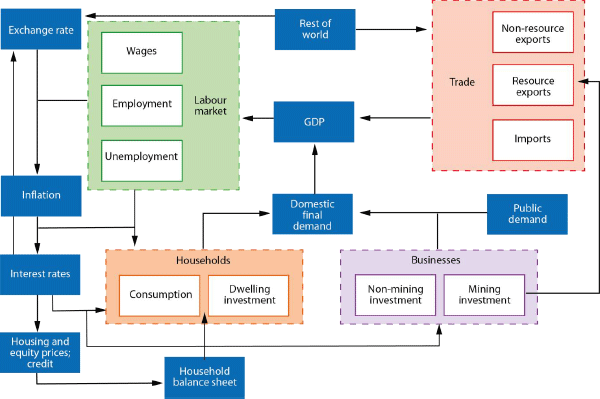
In MARTIN, the cash rate influences economic activity primarily through the exchange rate, dwelling investment, asset prices and the interest payments (and receipts) of households and businesses. Through these channels, a reduction in the cash rate provides a short-term boost to GDP growth because of increases in export volumes, dwelling investment, consumption and business investment and substitution in the composition of demand away from imported goods and services. Stronger GDP growth boosts household income, further increasing consumption and business investment. To expand capacity, firms must hire more workers, which increases employment and lowers the unemployment rate. Lower unemployment reduces the amount of spare capacity in the labour market and puts upward pressure on wage growth. Higher wages and import prices (because of exchange rate depreciation), in conjunction with increased capacity pressures, put upward pressure on inflation. Section 5.1 shows the effects of a change in interest rates on economic activity and quantifies the contribution of individual channels to the aggregate response.
3.2 Long-run Properties
To predict the behaviour of economic variables over a few months or quarters, it is often sufficient to extrapolate their recent trends into the future. However, one of MARTIN's core tasks is to provide a sense of how variables like inflation, GDP growth or the unemployment rate will evolve in scenarios or forecasts that span several years or even decades. Over these horizons, the model's projections will also reflect its long-run properties. If these long-run properties are implausible then the projections may lack credibility. For example, one might be sceptical about consumption forecasts from a model which predicted that, in the long run, nominal consumption expenditure grows faster than nominal GDP.
We impose a number of coefficient restrictions on MARTIN to ensure that its medium- and long-run projections are plausible. These restrictions ensure that the model converges to a stable balanced growth path, along which income and expenditure shares of GDP are stable, and variables like GDP growth, inflation and the unemployment rate converge to their target or potential values.
Four main assumptions ensure that MARTIN has a stable balanced growth path:
- The inflation rates of all price indices are equal in the long run. This ensures that relative prices also stabilise, but places no restrictions on the particular values at which they stabilise.
- Long-run income elasticities in the model's expenditure equations equal one. In conjunction with Assumption 1, this means that expenditure components of GDP, like consumption or services exports, grow at the same rate (in both real and nominal terms) in the long run, ensuring that the model's expenditure shares are constant.
- Nominal wages grow at the sum of inflation and labour productivity growth in the long run. This ensures that the wage and capital shares of income are stable.
- The central bank adjusts interest rates to ensure that consumer price inflation equals the inflation target and the unemployment rate equals the NAIRU.
While some of these assumptions are uncontroversial (for example, that the central bank adjusts interest rates to meet its inflation target) others (such as the assumption that long-run expenditure shares are constant) are open to debate. In cases where the coefficient restrictions are clearly at odds with the data, we allow for more flexible specifications, typically by including time-varying parameters or structural breaks in coefficients. But in most cases, we believe that our assumptions provide a better explanation for the long-run behaviour of Australian macroeconomic variables than alternatives that would allow factor and expenditure shares to expand and contract without bound.
The time it takes for MARTIN to converge to its long-run balanced growth path varies depending upon the current state of the economy or the scenario being considered. However, we typically find that most variables converge to their long-run paths within a decade.
4. Core Equations
In this section we describe the core behavioural equations in MARTIN. Our goal here is not to provide a comprehensive account of the full set of equations and identities, or the econometric details of the individual equations, all of which we provide in our online appendix. Rather, it is to highlight the economic intuition behind the key relationships that drive MARTIN's forecasts and scenarios.
In line with this goal, there are a number of small differences between the way in which we present individual equations in this section and the way in which they appear in MARTIN's code. One relates to the equations that take an error correction form. In describing these equations in the text, we make an explicit distinction between the long-run and short-run components. In practice, however, we estimate almost all of these equations using a one-step approach – that is, we estimate the short-run and long-run parts of the equations simultaneously. In addition, to simplify the presentation of the equations we omit terms that have no economic interpretation, such as dummy variables used to account for outlying observations.
Table 1 defines the variables used in the equations described below. To simplify notation, in the equations below we use capital letters to denote the level of a variable and lower case letters stand for the natural logarithm of a variable. The symbol refers to the quarterly change in the value of a variable. In all the ECM equations, the symbol is the speed of adjustment parameter and errort refers to the equilibrium error. The data used are quarterly. The estimation samples differ between equations. For most of the model's expenditure and labour market variables, such as consumption and the unemployment rate, our estimation samples begin in the 1980s or earlier. Using longer samples that include periods of heightened macroeconomic volatility helps us to pin down macroeconomic relationships that are harder to identify in the more stable economic environment that has existed since the early 1990s. In contrast, we estimate the equations of most of the nominal variables, including inflation and wages growth, over samples starting in the 1990s. This reflects structural breaks in many of these series that occurred around this time, which makes estimation over longer samples unreliable.[11]
| Variable | Definition | Specification | Value | Source |
|---|---|---|---|---|
| Trend and supply side | ||||
| pi_e | Inflation expectations | Per cent | RBA | |
| RSTAR | Neutral interest rate | Per cent | Real | RBA |
| ta | Trend labour productivity | Log | Real | RBA |
| thpp | Trend average hours worked | Log | RBA | |
| TLUR | NAIRU | Per cent | RBA | |
| tpop | Trend population | Log | RBA | |
| ty | Trend growth (for Okun's Law) | Log | Real | RBA |
| Household sector | ||||
| hcoe | Compensation of employees | Log | Real | ABS, RBA |
| hdy | Household disposable income | Log | Real | ABS, RBA |
| hnw | Household net wealth | Log | Real | ABS, RBA |
| hoy | Household non-labour disposable income | Log | Real | ABS, RBA |
| nhc | Household credit | Log | Nominal | ABS, APRA, RBA |
| nhfa | Household financial assets | Log | Nominal | ABS |
| rc | Household consumption | Log | Real | ABS |
| Housing sector | ||||
| id | Dwelling investment | Log | Real | ABS |
| kid | Dwelling stock | Log | Real | ABS, RBA |
| otc | Ownership transfer costs | Log | Real | ABS |
| ph | Housing prices | Log | Nominal | Corelogic, RBA |
| prt | Household rents | Log | Nominal | ABS |
| rph | Housing prices | Log | Real | ABS, Corelogic, RBA |
| Business sector | ||||
| IBCR | Cost of capital | Per cent | RBA | |
| ibn | Non-mining business investment | Log | Real | ABS |
| IBNDR | Non-mining depreciation rate | Per cent | ABS, RBA | |
| ibre | Mining investment | Log | Real | ABS |
| IBREDR | Mining depreciation rate | Per cent | ABS, RBA | |
| kibre | Mining capital stock | Log | Real | ABS |
| nibre | Nominal mining investment | Log | Nominal | ABS |
| Foreign trade and foreign sector | ||||
| m | Imports | Log | Real | ABS |
| tot | Terms of trade | Log | ABS | |
| xre | Resource exports | Log | Real | ABS |
| xs | Services exports | Log | Real | ABS |
| wy | Major trading partner GDP | Log | Real | RBA |
| Prices and labour market | ||||
| le | Employment | Log | ABS | |
| LUR | Unemployment rate | Per cent | ABS | |
| nulc | Nominal unit labour costs | Log | Nominal | ABS |
| nulcbs | Nominal unit labour costs with Balassa-Samuelson adjustment | Log | Nominal | ABS, RBA |
| p | Consumer price index | Log | Nominal | ABS |
| Prices and labour market | ||||
| pae | Average earnings from the national accounts | Log | Nominal | ABS, RBA |
| pex | Headline CPI excluding volatile items | Log | Nominal | ABS |
| poil | Oil price in Australian dollars | Log | Nominal | Bloomberg, RBA |
| ptm | Trimmed mean inflation | Log | ABS | |
| pw | Wage price index, excluding bonuses | Log | Nominal | ABS |
| rlc | Labour costs (average hourly earnings) | Log | Real | ABS |
| rulc | Real unit labour costs | Log | Real | ABS |
| Financial markets | ||||
| N2R | Two-year government bond rate | Per cent | Nominal | RBA, Yieldbroker |
| NBR | Business lending rate | Per cent | Nominal | RBA |
| NBRSP | Business spread to cash rate | Percentage points | Nominal | RBA |
| NCR | Overnight cash rate | Per cent | Nominal | RBA |
| NMR | Mortgage rate | Per cent | Nominal | RBA |
| NMRSP | Mortgage rate spread to cash rate | Percentage points | Nominal | RBA |
| peqi | Market price of equities | Log | Nominal | Bloomberg, MSCI, RBA, Refinitiv |
| RCR | Cash rate | Per cent | Real | RBA |
| rewi | Export-weighted exchange rate index | Log | Real | BIS, RBA |
| RMR | Mortgage rate | Per cent | Real | RBA |
| rtwi | Trade-weighted exchange rate index | Log | Real | RBA |
| WR2SP | Spread from Australian to G3 policy rates | Percentage points | Real | RBA |
| WR2SP_AVE | Average WR2SP since 1993 | Percentage points | Real | RBA |
| National aggregates | ||||
| AT | Net asset transfers between household and public sectors | Level | Real | RBA |
| g | Public demand | Log | Real | ABS |
| gne | Gross national expenditure | Log | Real | ABS |
| iad | Import-adjusted demand | Log | Real | RBA |
| ny | Gross domestic product | Log | Nominal | ABS |
| SD | Statistical discrepancy | Level | Real | ABS |
| V | Change in inventories | Level | Real | ABS |
| y | Gross domestic product | Log | Real | ABS |
| Implicit price deflators (IPD) | ||||
| pc | Household consumption IPD | Log | ABS | |
| pdfd | Domestic final demand IPD | Log | ABS | |
| pgne | Gross national expenditure IPD | Log | ABS | |
| pibn | Non-mining business investment IPD | Log | RBA | |
| pibre | Mining business investment IPD | Log | RBA | |
| pid | Dwelling investment IPD | Log | ABS | |
| pm | Imports IPD | Log | ABS | |
| pmcg | Imported consumption goods IPD | Log | ABS | |
| pxre | Resource exports IPD | Log | ABS | |
| py | Gross domestic product IPD | Log | ABS | |
4.1 The Supply Side
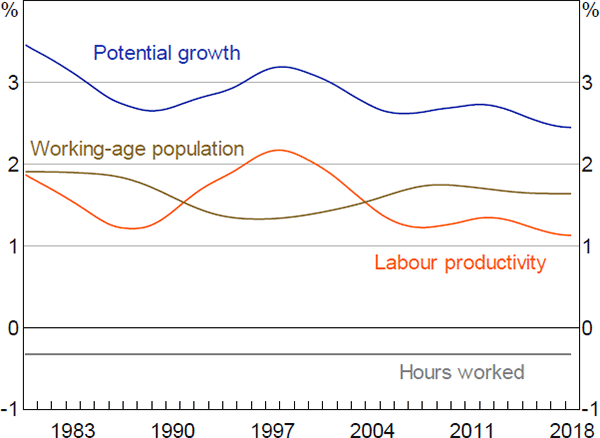
The supply side of the model consists of exogenous processes governing the evolution of trend labour productivity growth, trend population growth and trend average hours worked.[12] Together, these variables determine the potential growth rates of GDP, employment and real wages.
The log of trend labour productivity, tat, follows a random walk with drift, . The drift term is an AR(1) process that mean-reverts at a 5 per cent quarterly rate:
where is the long-run mean of labour productivity growth. We restrict the coefficient on the lag of the drift term to equal 0.95. This ensures that the drift term accounts for persistent variation in productivity growth, while still having a well-defined mean. An alternative would be to allow trend productivity growth to follow a random walk (by setting the coefficient on lagged productivity growth equal to one). In practice, this would produce similar estimates of trend productivity growth over history. However, it would make the model unstable in simulations because productivity growth could increase or decrease without bound.
The log of trend population, tpopt, also follows a random walk with drift, . The drift term is an AR(1) process that mean-reverts at a 5 per cent quarterly rate:
where is the long-run mean of population growth.
The log of trend average hours worked, thppt, follows a random walk with drift, . Unlike productivity and population growth, we restrict the long-run drift of hours worked to converge to a mean of zero at a 5 per cent quarterly rate. This ensures that in long-run projections the decline in hours worked observed over recent decades eventually comes to an end.
In the current version of MARTIN, we set long-run annual labour productivity growth to 1.5 per cent and long-run annual population growth to 1.25 per cent, meaning that the economy's long-run potential growth rate is 2.75 per cent.
Because aggregate supply ultimately determines the growth rates of income and expenditure, the supply-side trends enter many of the equations in MARTIN. As such, we need to derive values for these variables over history. To do so, we assume that the measured values of labour productivity, population and hours worked in the data equal their long-run trends plus a random error term, estimate the parameters of the models via maximum likelihood, and then conditional on those parameter estimates use a Kalman filter to infer the value of the long-run trends given the data. In estimation we restrict the standard deviation of the error in the drift terms to be 1 per cent of the standard deviation of the errors in the level equations. This ensures that the drift terms capture low frequency changes in the value of these series without overfitting the data.
Figure 2 plots the estimated trends and the economy's implied potential growth rate in annualised terms. Trend population growth averaged around 1¾ per cent in the 1980s and 2010s, and around 1½ per cent between those times. Trend labour productivity growth declined during the 1980s, increased during the 1990s and has since settled at around 1¼ per cent. The decline in average hours worked has made a small subtraction from potential growth over recent decades. Summing these trends together, we estimate that potential GDP growth averaged a bit over 3 per cent between the early 1980s and early 2000s and has declined slightly to around 2¾ per cent since then.
Sources: ABS; Authors' calculations; RBA
4.2 Consumption and the Household Sector
4.2.1 Consumption and household income
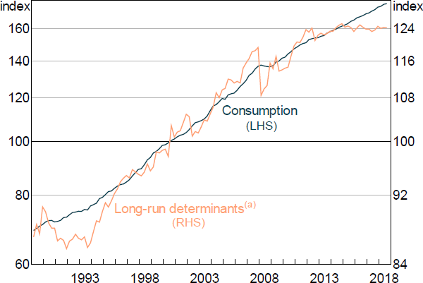
The consumption equation captures the spending and saving decisions of households. We model consumption within a permanent income hypothesis framework, which implies a long-run relationship between consumption, household income and net wealth (Figure 3).[13] This relationship can also be motivated as the linearisation of the household sector's budget constraint (Lettau and Ludvigson 2001). To ensure that consumption grows at the same rate as income and net wealth along a balanced growth path, we restrict the coefficients on these variables to sum to one. We also include the real interest rate in the long run part of the equation to capture the idea that it is optimal for households to save a larger proportion of their income when real interest rates are high. We impose a small coefficient on this latter variable, which implies that a 100 basis point decrease in interest rates raises the long-run level of consumption by 0.05 per cent. We also include a level shift in the long-run equation that occurs in 2007:Q1. This captures an observed shift in the household saving rate, conditional on the levels of income and wealth, which occurred at this time.
Consumption deviates from its long-run equilibrium due to short-run movements in labour and non-labour income and net wealth. Along a balanced growth path, the economy's trend growth rate (which is the sum of trend labour productivity growth, population growth and growth in hours worked) also influences consumption. In this way, the equation allows for the possibility that some households make their consumption decisions based on long-run income expectations while the expenditure of other households, possibly because they face collateral or liquidity constraints, is more sensitive to current income. Because the model's estimates of trend labour productivity and population growth are time-varying, the equation should be robust to changes in trend growth over time. We also include the change in the unemployment rate to capture the precautionary savings motive induced by economic uncertainty, as well as to account for the possibility that changes in the unemployment rate alter the distribution of income, and hence consumption, in ways that aggregate household income does not capture (Muellbauer and Williams 2011).
Note: (a) Includes household income, net wealth and the cash rate
Sources: ABS; Authors' calculations
4.2.2 Household balance sheet
The net wealth of households is made up of their assets less their liabilities. We model each of these quantities in nominal terms. Household assets consist of non-financial and financial assets. The growth rate of non-financial assets is linked to the growth rate of the value of the housing stock, that is, housing prices times the housing stock. We model the housing stock using a standard capital accumulation equation in which next quarter's housings stock equals the undepreciated component of this quarter's housing stock plus gross dwelling investment. The housing price and dwelling investment models are described in Section 4.3.
The equation for household financial assets assumes that households hold a constant proportion of their portfolio in risky assets (Merton 1969).[14] This leads to an error correction specification where financial assets and equity values move together in the long run:
To ensure a stable long-run ratio between financial assets and equity values, we restrict the coefficient on equity values to equal one. In the short run, trend real growth and movements in equity prices also influence financial assets. We model equity values as expected earnings for listed firms divided by the earnings yield. Expected earnings depend largely on aggregate profits and commodity prices, while the earnings yield is related to the gap between the required rate of return on equities (proxied by the business lending rate) and the economy's trend growth rate.
The household sector's liabilities consist of liabilities to the financial sector (that is, household credit) and household debt outside the Australian banking system. In the long run, the stock of household credit is determined by the value of housing assets and the average loan-to-valuation ratio of housing loans. We proxy for the latter with the real mortgage interest rate, which captures the tendency for loan-to-valuation ratios to increase when real mortgage rates decline.
In the short run, the growth rate of nominal household credit depends on housing price growth, growth in the dwelling stock, changes in mortgage interest rates and the rate of inflation. The coefficient restrictions ensure that the stock of credit grows at the same rate as nominal GDP along the model's balanced growth path.
Household debt outside the banking system is a volatile series and hard to account for using standard macroeconomic data. Because of this, we model this component of liabilities as an autoregressive process, constraining its mean growth to equal the rate of trend nominal GDP growth along a balanced growth path.
4.3 The Housing Sector
The dwelling investment, housing price and rents equations capture the demand for and supply of housing services. The behavioural dynamics underlying these equations reflect households' decisions about whether to buy, sell or build dwellings.
4.3.1 Dwelling investment
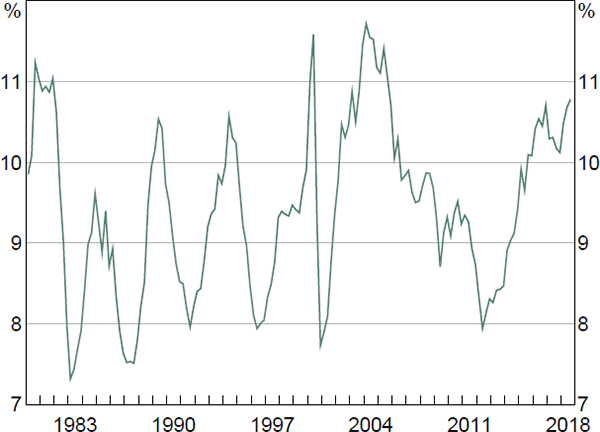
We model dwelling investment using an ECM with consumption, real mortgage interest rates and the relative price of dwelling investment. In the long run, households are assumed to allocate a stable share of their expenditure to housing and non-housing consumption, conditional on the level of interest rates. This implies that the ratio of nominal dwelling investment to nominal consumption expenditure will fluctuate around a constant mean, which is strongly evident in the data (Figure 4). A decrease in real interest rates lowers the cost of borrowing to construct new housing as well as the cost of new housing relative to established housing (whose price tends to rise with lower interest rates). This makes dwelling investment more profitable and raises its expenditure share relative to consumption.
Dwelling investment can deviate from its long-run equilibrium because of short-run movements in the nominal mortgage interest rate and real housing prices. Along a balanced growth path, real dwelling investment grows at the economy's trend growth rate.
Sources: ABS; RBA
4.3.2 Housing prices
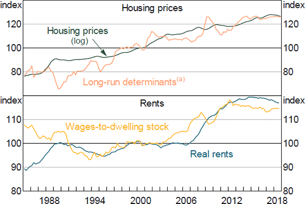
We model housing prices using an ECM similar to that in Fox and Tulip (2014). Housing prices are expected to tend towards their fundamental value, which is the price where households are indifferent between owning and renting. We assume that variation in the user cost of owning a home is driven by movements in the real mortgage interest rate.[15] In the long run, if the real mortgage rate is constant, nominal housing prices will grow in line with rents. Like Fox and Tulip, we find that the rents–user cost framework can account for much of the growth in housing prices over recent decades (Figure 5).
In the short run, changes in housing prices have a large inertial component, and are also influenced by recent movements in nominal mortgage interest rates.
Note: (a) Includes CPI rents and the real cash rate
Sources: ABS; Authors' calculations; Corelogic
4.3.3 Rents
In the long run, real rents depend on the demand for and supply of housing. We measure the demand for housing using real compensation of employees – the wage component of real household income. The supply of housing is given by the housing stock. This relationship can account for a large part of the low frequency movement in rents over recent decades (Figure 5). Because rent inflation is a highly persistent series, much of its short run behaviour is accounted for by its own lag.
4.4 Business Investment
We model non-mining and mining investment separately, reflecting the fact that the determinants and historical behaviour of these two series differ substantially.
4.4.1 Non-mining business investment
The long run component of the non-mining business investment equation is based on neoclassical investment theory, which asserts that firms invest to the point where the marginal return on an additional unit of capital is equal to its user cost (Jorgenson 1963). In MARTIN, this is captured by a long-run relationship between investment, output and the cost of capital. We use gross national expenditure (GNE) as our measure of output, rather than GDP, because it abstracts from large movements in resource export volumes, which are unlikely to create demand for non-mining investment. However, we include the mining investment share of GDP as an additional variable to capture the tendency for expansions in the resources sector to draw resources away from other parts of the economy. In most theoretical models, the steady-state investment-to-output ratio is a function of trend GDP growth and the capital depreciation rate. Therefore, we also include these variables in the equation.
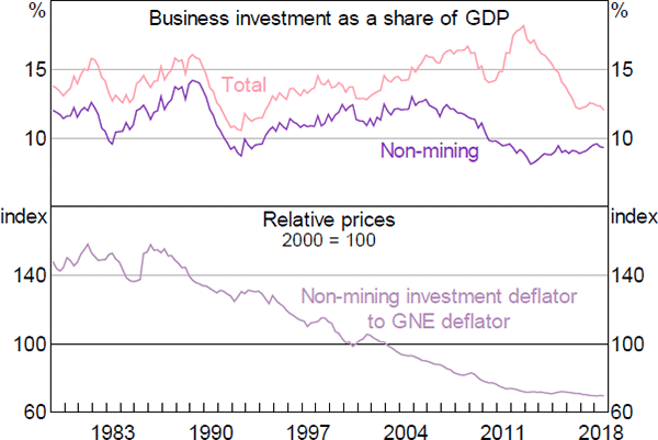
Any empirical investment equation using Australian data must reconcile three stylised facts: (i) the ratio of nominal business investment to GDP has had a reasonably stable mean over recent decades; (ii) the relative price of business investment (which is a component of the cost of capital) has declined substantially over this time; and (iii) most time series estimates suggest that the direct response of investment to changes in interest rates (another component of the cost of capital) is small (Figure 6). To account for these features of the data, we separate the relative price of non-mining business investment from other components of the cost of capital and impose a coefficient of −1 on the former.[16] This coefficient restriction means that changes in the relative price of investment goods do not alter the investment share of GDP in the long run. We calibrate the coefficient on the other components of the cost of capital to equal –0.4, which is consistent with a range of overseas and Australian evidence (Antràs 2004; Cockerell and Pennings 2007), as well as with the coefficient on real wages in MARTIN's employment equation.[17]
Quarterly changes in non-mining business investment are volatile and hard to explain using macroeconomic data. Reflecting this, the short run component of the equation is parsimonious, only including the two-quarter change in GNE.
Sources: ABS; Authors' calculations
4.4.2 Mining investment
Resource firms produce undifferentiated products and take the prices of these products as given. These prices (equal to the world price of resources, adjusted for the value of the Australian dollar exchange rate), relative to the prices of non-resource goods and services, dictate the size of the resources sector. A rise in resource export prices increases the size of the resources sector, and hence the mining investment share of GDP. Holding relative resource export prices fixed, this share converges to a stable value in the long run, which depends on the economy's trend growth rate as well as the depreciation rate of capital in the resources sector. In the short run, the growth rate of resource exports depends positively on recent changes in relative resource export prices and the economy's trend growth rate.
4.5 Foreign Trade
We disaggregate exports into five categories – services, manufactures, agricultural, resources and other – reflecting the different determinants and trends in these series. In contrast, we model imports at the aggregate level.
4.5.1 Non-resource exports
The non-resource exports equations share a common structure. In the long run, each component of exports depends on overseas demand, measured as the export-weighted GDP of Australia's major trading partners, and relative prices, measured as the real export-weighted exchange rate. An increase in overseas demand raises export volumes, whereas an increase in the relative price of goods and services produced in Australia lowers exports. We constrain the demand elasticities to equal one, but estimate the price elasticities. The price elasticities turn out to differ substantially between export components.
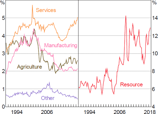
Global trade liberalisation, lower transport costs and other related developments have led to substantial changes in the ratio of exports to GDP over the past thirty years that cannot be fully accounted for by growth in foreign GDP or changes in relative prices. These shifts in trade shares are particularly evident in exports of services and manufacturing products (Figure 7). To account for these features of the data, we include time-varying constants in the manufactured and services exports equations. We estimate these constants using state-space methods.[18] In the short run, growth in exports generally depends on growth in foreign demand and changes in relative prices.
For example, the equation for services exports is:
Time-varying constant:
As the equations for the remaining categories of non-resource exports are similar to that of services exports, we leave the precise specifications of these equations to the Online Appendix.
Sources: ABS; RBA
4.5.2 Resource exports
In the long run, resource exports are determined by the supply of mining output. We assume that mining supply is proportional to the capital stock of the resources sector, reflecting the fact that production of mining commodities is highly capital intensive. Mining capital affects exports with a lag, because there is often a delay between the installation of new capital and the time when it starts to produce output.
Resource exports volumes vary considerably from quarter to quarter, often because of supply shocks that temporarily reduce output, as well as the lumpy nature of new production. Because of this, the coefficient on lags of resource exports is negative – a decrease in resource exports growth in one quarter is likely to be partially unwound in the subsequent quarter.
4.5.3 Imports
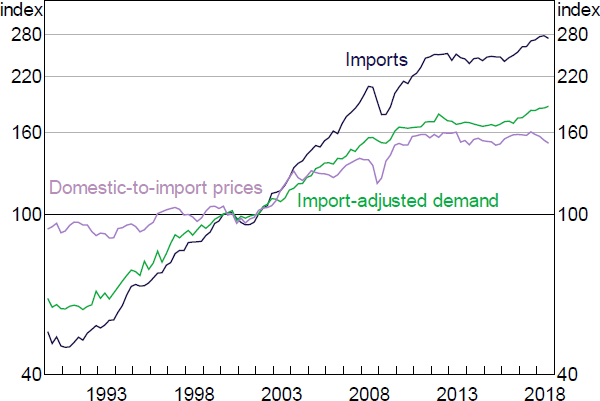
In the long run, import volumes depend on the level of domestic demand and the relative price between imports and goods and services produced in Australia (Figure 8). We use an import-adjusted measure of demand that weights each component of domestic final demand by its relative import intensity.[19] So, for example, an increase in business investment – which is relatively import intensive – will cause a larger increase in imports than a similar-sized increase in dwelling investment – which has a low import intensity. The relative prices term is the ratio of the import price deflator to the domestic final demand deflator. The estimated coefficient on this term is close to –1. This is consistent with the fact that the ratio of nominal import values to nominal GDP has been broadly stable over the estimation sample. However, it has the implication that import volumes respond quickly to exchange rate movements, which seems at odds with the observation that exchange rate pass-through to domestic prices occurs with a significant delay (Chung, Kohler and Lewis 2011). To reconcile these two stylised facts, we include the average of four lags of relative import prices in the long run part of the equation. This limits the speed with which changes in import prices translate into import volumes, and also prevents temporary exchange rate movements from driving large changes in imports. The long-run properties of the model, however, are unaffected by this modelling choice. In the short run, imports growth is a function of contemporaneous and lagged demand and relative prices.
Sources: ABS; Authors' calculations
4.6 National Accounts Aggregates
We construct the national accounts aggregates – gross domestic product, gross national expenditure and domestic final demand – by summing the expenditure components described above. For nominal values this summation exactly matches the published aggregates. But for the chain volume expenditure components, the summation only approximates to the published aggregates when relative prices change. In practice, these approximation errors are typically small, particularly for forecasts and scenarios constructed close to the national accounts reference year. Although more complex aggregation methods are possible, we found that simple aggregation introduces less bias in the forecasting process than these alternative approaches.
4.7 Prices and Wages
The prices and wages block of the model links the real and nominal sides of the economy. Developments in this block have a large influence on monetary policy settings and feed back into other aspects of the model, such as household income.
There are two main equations in the prices and wages block. The first is the equation for the wage price index (WPI). The WPI captures pure wage effects, abstracting from compositional changes in employment and labour quality. We map the WPI into average earnings from the national accounts (AENA), which incorporates compositional shifts and changes in labour quality and is the relevant wage measure for the determination of household income and prices (Figure 9). In turn, AENA feeds into nominal unit labour costs, and then into prices through the trimmed mean inflation equation, which is the second main equation in the prices and wages block.
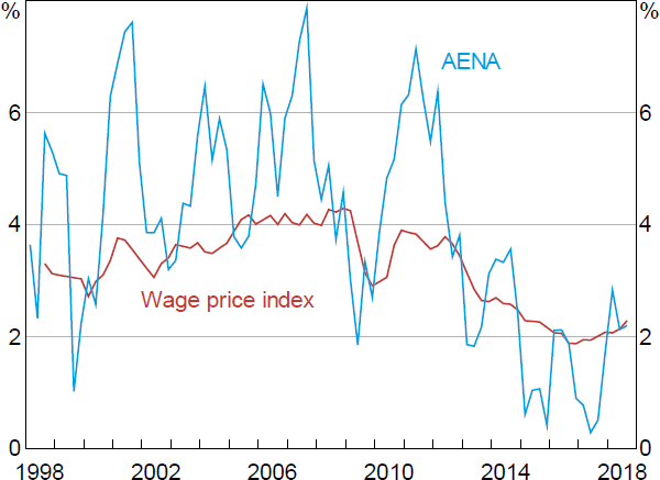
Sources: ABS; RBA
Many of MARTIN's price and wage variables are influenced by the NAIRU and inflation expectations. Both of these variables are exogenous in the model and, as neither can be observed directly, are instead constructed using the approach described in Cusbert (2017).
4.7.1 Wage price index
We model the WPI using a Phillips curve approach. Less spare capacity in the labour market, as measured by a decreasing unemployment rate and smaller unemployment gap, will lead to faster wages growth. Higher inflation expectations and faster growth in the GDP deflator also raise wages growth, as nominal wages will need to increase more quickly to maintain a given real wage. An increase in productivity growth also leads to faster wage growth, because it raises the marginal product of labour.
Along a balanced growth path, the unemployment rate will converge to the NAIRU and inflation expectations and growth in the GDP deflator will converge to 2.5 per cent. When this occurs, growth in the WPI will reflect two factors: prices growth of 2.5 per cent; and real WPI growth, which will be proportional to labour productivity growth. However, real WPI will grow more slowly than aggregate labour productivity, because the WPI is partly quality adjusted.
4.7.2 Average earnings from the national accounts (AENA)
We map the WPI into AENA using the following equation:
Faster growth in the WPI feeds through to AENA. The pass-through is greater than one-for-one, because AENA tends to be more cyclical than the WPI. Along a balanced growth path, AENA grows at the sum of labour productivity growth plus inflation.
4.7.3 Trimmed mean inflation
We model trimmed mean inflation using a mark-up model, similar to the specification described in Norman and Richards (2012). In the long run, firms are assumed to set their prices as a fixed mark-up over their input costs. As such, there is a long-run relationship between the price level, nominal unit labour costs and the price of imported consumption goods (Figure 10).[20] If prices are unusually low relative to input costs, we should expect inflation to be higher than usual as firms seek to restore mark-ups to their desired level. Similarly, if prices are unusually high relative to input costs, we should expect inflation to be lower than usual.
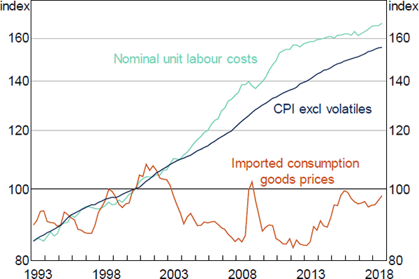
Sources: ABS; RBA
We restrict the coefficients on unit labour costs and import prices to sum to one. This condition, known as static homogeneity, ensures that the model has the desirable steady-state property that if all input costs were to double, consumer prices would also double in the long run, preventing long-run drift in mark-ups. Two aspects of our specification are necessary for this restriction to fit the data. First, we use the headline consumer price index (CPI) excluding volatile items as our measure of the price level in the long run part of the equation, rather than the trimmed mean price index, as the former is the more relevant measure of output prices in the mark-up framework.[21] Second, like Stone, Wheatley and Wilkinson (2005), we make a small adjustment to the economy-wide unit labour costs variable to account for the fact that labour costs associated with the production of exports (which typically exhibit faster productivity growth than unit labour costs associated with the production of domestically consumed goods and services) do not feed into domestic inflation.[22] With these variables, the restriction that the coefficients on unit labour costs and import prices sum to one cannot be rejected at standard significant levels.
We allow for the possibility that mark-ups might vary systematically over the economic cycle by including the unemployment gap in the equation. The coefficient on the unemployment gap is negative, indicating that inflation and mark-ups will tend to be lower when the unemployment rate is higher. That is, mark-ups are procyclical.
4.7.4 CPI inflation
We model headline CPI inflation as a function of trimmed mean inflation and oil prices. Doing so accounts for the sizeable direct effect oil prices can have on headline inflation by influencing automotive fuel prices, which are often trimmed out of trimmed mean inflation. We model inflation in consumer prices excluding volatile items as trimmed mean inflation plus an error term.
4.8 Labour Market
4.8.1 Employment
In the long run, employment is determined by a standard labour demand equation that depends on output, the real wage and labour productivity (Figure 11).[23] The equation is similar to those described in Debelle and Vickery (1998) and Hutchings and Kouparitsas (2012). Along a balanced growth path, the wage share is stable and employment grows at the rate of output growth less growth in labour productivity and average hours. This relationship implies a long-run coefficient of one on output, and negative one on trend productivity and average hours. The coefficient on the wage share represents the elasticity of substitution between labour and capital, which indicates how much employment will respond to changes in real wages that cannot be explained by productivity.
In the short run, employment growth has an inertial component and also depends on the recent growth rates of labour costs and GDP. We address concerns of endogeneity in the contemporaneous output and real wages growth terms by estimating the equation using instrumental variables, using lags of the growth of the unemployment rate and labour costs as instruments.
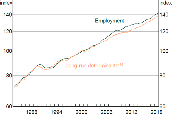
Note: (a) Includes wage share and trend growth variables
Sources: ABS; Authors' calculations
4.8.2 Unemployment rate
We model the unemployment rate using the Okun's Law approach described in Lancaster and Tulip (2015). This relates changes in the unemployment rate to changes in GDP growth relative to a time-varying trend. The change in the unemployment rate also contains an inertial component and depends additionally on growth in real unit labour costs. The latter variable captures the tendency for firms to substitute away from labour when that factor of production becomes more expensive.
As in Lancaster and Tulip, we use a state-space model to estimate time-varying coefficients on lags of changes in the unemployment rate and trend GDP growth. In estimation, we assume that both of these trends follow a random walk.
We project changes in the unemployment rate using the estimated measurement equation from the state-space model. In projections, we hold constant at its last estimated value. The measure of trend growth in the unemployment equation, tyt, is the growth rate that keeps the unemployment rate constant. This rate can differ from the definition of potential GDP growth described in Section 4.1. In forecasts and projections, we converge tyt from its final value towards the standard definition in the model, which is the sum of growth in labour productivity, population and average hours.
4.9 Interest and Exchange Rates
4.9.1 Monetary policy reaction function
In light of the well-known difficulties in estimating the parameters of monetary policy reaction functions (Mavroeidis 2010), MARTIN's baseline specification features a calibrated reaction function in which the overnight cash rate responds to year-ended inflation, the unemployment gap and the change in the unemployment rate:
The variable RSTARt is the time-varying neutral interest rate, which is constructed using the approach described in McCririck and Rees (2017). This variable accounts for much of the decline in the real cash rate over recent decades.
We use the unemployment gap as a measure of spare capacity rather than the output gap for three reasons. First, the unemployment gap is conceptually closer to the RBA's mandated objective of full employment than the output gap. Second, in practice most of the variation in Australian output gap measures comes from variation in the unemployment gap. Third, the unemployment gap is arguably better measured than the output gap. We choose the parameters of the reaction function to provide a reasonable description of the change in the cash rate during several key economic episodes over the past 25 years, including the 1994–95 tightening cycle, the Asian financial crisis and the global financial crisis.
4.9.2 Other interest rates
Changes in the cash rate influence economic activity and inflation largely through their effect on other interest rates in the economy. The most important interest rates in MARTIN are mortgage rates, business lending rates and two-year government bond yields.
The mortgage interest rate is equal to the cash rate plus an interest rate spread. The spread follows an AR(1) process. We include a break in the mean of this spread in early 2008, to capture the increase in mortgage interest rates that occurred following the global financial crisis.
The business lending rate is equal to the cash rate plus an interest rate spread. The spread follows an AR(1) process and also depends on the level of the unemployment gap. The latter variable accounts for the fact that business lending spreads tend to be countercyclical.
Two-year government bond yields depend on the current level of the cash rate and expectations of its future level (proxied by the neutral real interest rate plus inflation expectations):
Real interest rate measures appear in many of MARTIN's equations. We calculate these measures by adjusting nominal interest rates for year-ended trimmed mean inflation.
4.9.3 Real trade-weighted index
We model the real trade-weighted index (TWI) exchange rate using an ECM framework as in Hambur et al (2015). In the long run, there is a cointegrating relationship between the real TWI, the terms of trade and the spread between Australian and G3 real two-year government bond rates. In the short run, changes in the terms of trade and the government bond spread also influence the real exchange rate.
4.10 Foreign Sector
MARTIN's foreign sector is parsimonious and is made up of a small number of exogenous variables, including major trading partner (MTP) GDP growth, various world prices and the interest rates of major advanced economies. These foreign variables affect domestic variables such as exports, imports and the real TWI.
In the long run, we assume that the growth rate of real MTP GDP converges to Australia's trend GDP growth rate. Similarly, growth in foreign prices converges to the Australian inflation target. Foreign policy rates converge to an exogenous estimate of the foreign neutral interest rate, while longer-term interest rates converge to the policy rate plus an estimated term premium.
The foreign block is another area where a tension arises between matching the data and ensuring desirable model properties. For example, the restriction on foreign economic growth is strongly at odds with recent history – on a trade-weighted basis, the GDP growth rates of Australia's major trading partners have exceeded Australian GDP growth over recent decades. However, for a stable balanced growth path to exist either the growth rate of foreign GDP must converge to the growth rate of domestic GDP or relative prices between Australian and foreign goods must drift at a rate that exactly offsets the growth differential.[24] Imposing a slow convergence of foreign GDP growth to Australian GDP growth turned out to be a simpler approach, with fewer implications for the model's dynamic properties, than imposing arbitrary restrictions on the drift of relative prices and the size of trade price elasticities.
While including a more sophisticated foreign sector in MARTIN would have some advantages, we favoured a simpler approach because MARTIN is intended to be a model of the Australian economy. When and if we need more detail on foreign variables, we can supplement MARTIN with other models that have more developed foreign sectors.[25]
5. Model Dynamics
In this section, we describe some of the dynamic properties of MARTIN. We first show the responses of key macroeconomic variables to three exogenous innovations, or shocks: an increase in the cash rate, a depreciation of the real exchange rate and a fall in housing prices. To provide some context for the results, we compare MARTIN's responses in the cash rate and exchange rate exercises to those from the RBA's DSGE model, MSM. We then compare the unconditional moments of some of MARTIN's key variables to their empirical counterparts.
5.1 An Increase in the Cash Rate
Figure 12 shows the responses of key aggregate variables to a 100 basis point increase in the cash rate that persists for four quarters, after which the cash rate follows its standard reaction function. The increase in the cash rate translates into higher mortgage and business lending rates, which raises borrowing costs for firms and households. It also leads to an appreciation of the real exchange rate. The net effect is to lower the level of GDP by around 0.8 per cent six quarters after the shock. The lower level of economic activity translates into an increase in the unemployment rate, which rises by 0.3 percentage points. The decline in aggregate demand and weaker labour market conditions contribute to a reduction in wages growth and inflation, which fall by a little less than 0.2 percentage points in year-ended terms after two years.
The GDP response to higher interest rates in MARTIN is similar to the response in MSM. However, the declines in wages growth and inflation in MARTIN are smaller than in MSM, and occur with a lag. In MSM, firms are forward looking and respond to the anticipated fall in demand after an increase in the cash rate by lowering their prices. In MARTIN, inflation does not decline until the contraction in demand translates into a rise in the unemployment rate and a fall in input costs.
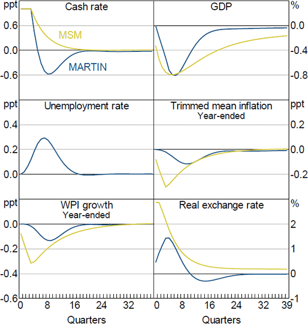
Sources: Authors' calculations; RBA
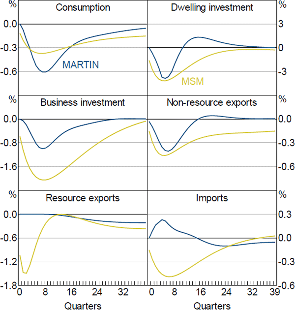
In common with other Australian macroeconomic models (Lawson and Rees 2008; Gibbs et al 2018), dwelling investment is the most interest-sensitive component of expenditure in MARTIN, declining by slightly more than three per cent following a 100 basis point increase in the cash rate (Figure 13). Household consumption declines by a bit less than GDP. However, because it accounts for a large share of expenditure, consumption makes a large contribution to the overall contraction in economy activity. The declines in consumption and dwelling investment in MSM are broadly similar to those in MARTIN, although MSM's responses are somewhat more persistent.
In MARTIN, business investment declines by about as much as GDP following an increase in interest rates. At first glance, the size of this response is somewhat surprising, as previous research has indicated that Australian firms' investment decisions are not sensitive to changes in interest rates (Lane and Rosewall 2015). It turns out that this is also the case in MARTIN; the direct response to increased funding costs accounts for only a quarter of the total decline in business investment. The rest of the investment response is due to lower aggregate demand, which reduces firms' incentives to invest. Funding costs play a larger role in determining investment in MSM, and in that model business investment declines by twice as much as in MARTIN.
Sources: Authors' calculations; RBA
The response of exports and imports to interest rates is a key difference between MARTIN and MSM. In MARTIN, non-resource exports decline by around 0.3 per cent following the increase in interest rates, while imports increase by around 0.25 per cent. Both responses are largely due to the appreciation of the real TWI, which reduces the international competitiveness of Australian-produced goods and services; the increase in imports is partly mitigated by the contraction in domestic demand. Although the response of non-resource exports volumes in the DSGE model is similar to the response in MARTIN, in MSM import volumes also decline.
The contrasting response of imports in the two models reflects differences in the speed of exchange rate pass-through. The relevant price for determining import volumes in MARTIN is the import price deflator. This captures ‘first-stage’ exchange rate pass-through (that is, the response of import prices at the docks to exchange rate changes). Exchange rate movements typically move the import price deflator one-for-one within a couple of quarters. Import volumes are estimated to be highly responsive to this relative price. In MSM, import volumes depend on ‘second-stage’ exchange rate pass-through (that is, the response of the prices faced by households and firms to changes in the exchange rate). Second-stage pass-through is generally estimated to occur slowly and to be incomplete (Chung et al 2011; Burstein and Gopinath 2014). Because of this, in MSM the income effect of lower aggregate demand overwhelms the price effect of the appreciation and import volumes decline. Better understanding the behaviour of import volumes following exchange rate movements would be a useful avenue for future research.
The response of resource exports also differs between the two models. In MARTIN, resource exports initially do not respond to the increase in interest rates because the productive capacity of the resources sector is unchanged in the short run. Over time, however, the appreciation of the Australian dollar means that some marginal investment in the resources sector does not occur. As a result, resource exports decline slightly after a few years. In MSM, resource firms can alter their production in the short run and so output falls immediately after a rise in interest rates.
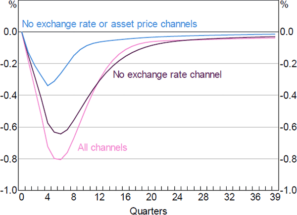
Figure 14 gives a sense of the relative contributions of the different channels of monetary transmission to the response of economic activity.[26] The line labelled ‘All channels’ replicates the response of GDP to the 100 basis point increase in the cash rate shown in Figure 12. In the line labelled ‘No exchange rate channel’ we impose the same interest rate path, but hold the real exchange rate fixed at its initial level. With this restriction, the level of GDP falls by around 0.6 per cent below its baseline level, compared to 0.8 per cent in the ‘All channels’ case. This indicates that the exchange rate channel accounts for around a quarter of the total effect of monetary policy on GDP. In the line labelled ‘No exchange rate or asset price channels’, we once again hold the exchange rate fixed and also turn off the response of housing and equity prices. In this case, the fall in GDP is close to 0.3 per cent, indicating that the asset pricing channel accounts for close to half of the overall GDP response to changes in interest rates. The remaining GDP response to interest rate changes reflects the other channels of monetary policy transmission, including the cash flow channel and the intertemporal substitution channel.
Sources: Authors' calculations; RBA
5.2 A Real Exchange Rate Depreciation
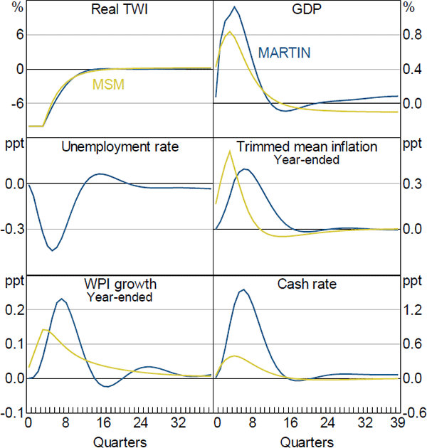
Figure 15 shows the responses of six key aggregate variables to a transitory 10 per cent real exchange rate depreciation. The depreciation reduces the price of Australian-produced goods and services relative to goods and services produced overseas. The resulting increase in demand for Australian goods and services raises the level of GDP by around 1 per cent after one to two years and lowers the unemployment rate by 0.4 percentage points. The expansion in economic activity and fall in the unemployment rate leads to an increase in wages growth. Increased wages growth and an increase in the price of imported goods and services raise firms' costs. In conjunction with the increase in demand, this leads to higher inflation, which rises by 0.3 percentage points. Higher inflation and a lower unemployment rate lead to an increase in the cash rate.
Sources: Authors' calculations; RBA
The responses of GDP, inflation and wages in MSM are all similar to those in MARTIN, although the pick-up in wages growth and inflation once again occur more quickly in MSM. The increase in the cash rate is also smaller in MSM. The differences in timing between the two sets of responses are in part due to the importance of expectations in MSM. Because households and firms in MSM are forward looking, they realise that the depreciation of the exchange rate will be inflationary and immediately adjust their wage demands and prices in response.
5.3 A Fall in Housing Prices
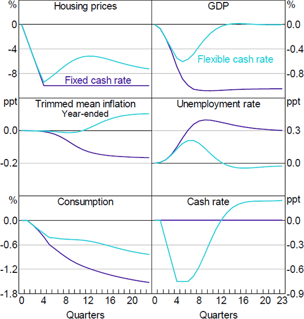
Figure 16 shows the responses of key aggregate variables to a persistent 10 per cent exogenous fall in housing prices. A decline in housing prices reduces the level of economic activity and inflation. In the absence of offsetting positive developments, the lower inflation and higher unemployment rate this implies could lead to a reduction in interest rates. To isolate the effects of lower housing prices from the effects of lower interest rates, we show two sets of results. In the first, we hold the cash rate fixed at its initial level. This shows the effects of lower housing prices independently of monetary policy. In the second, we impose an interest rate path that returns the level of economic activity to its previous trend after two to three years.
Sources: Authors' calculations; RBA
Lower housing prices affect the economy in several ways. Because housing is the largest component of household assets, lower housing prices reduce household net wealth, which lowers consumption. Lower housing prices also make new home building less profitable, which reduces dwelling investment. The decline in consumption and dwelling investment lowers aggregate demand, which reduces the incentives for firms to invest. The net effect, absent an interest rate response, is to lower the level of GDP by a bit more than 1 per cent below its baseline level after one to two years. The decline in economic activity reduces the demand for labour and causes the unemployment rate to increase by around 0.4 percentage points. The decline in economic activity and the higher unemployment rate leads to a fall in inflation of around 0.2 percentage points in year-ended terms.
The implications of lower housing prices are considerably smaller if monetary policy responds. The model's endogenous reaction function delivers a relatively slow interest rate response because it takes several quarters for inflation and the unemployment rate to respond to the fall in housing prices. However, because changes in housing prices are readily observable and strongly persistent, making the macroeconomic consequences predictable, this delayed response strikes us as unrealistic.[27] Therefore, the particular cash rate path that we consider involves a 75 basis point reduction in interest rates over four quarters following the decline in housing prices, after which monetary policy follows its standard reaction function.[28] This cash rate profile roughly halves the peak effect of lower housing prices on GDP and the unemployment rate, and returns these variables to their baseline trends within three years.
The reduction in the cash rate also raises housing prices relative to the scenario with a fixed cash rate. However, housing prices remain well below their initial level. This reflects the fact that monetary policy targets inflation and full employment, not asset prices. By limiting the decline in housing prices, monetary policy helps to support the level of economic activity. But other channels, such as the exchange rate channel and the intertemporal substitution channel are also at work. In practice, much of the recovery in GDP reflects an increase in export volumes and decrease in imports; even with a lower cash rate the level of consumption remains considerably below its baseline level following a persistent fall in housing prices.
5.4 Unconditional Moments
Another way to test the model's properties is to examine how well it can replicate key empirical features of the data, such as the means and standard deviations of macroeconomic variables. To calculate these moments in MARTIN, we run a large number of simulations. In each simulation we draw a selection of the reduced form residuals from the model's equations and impose these residuals on the model. We use a block bootstrap to draw the model residuals, which preserves the cross-variable and across-time correlation structure of the residuals observed in the data. After each simulation, we calculate the means and standard deviations of the model variables. Repeating this process for a large number of simulations gives us an indication of the unconditional moments of variables in the model.
Table 2 compares the unconditional means and standard deviations of selected variables in MARTIN to those in the data.[29] In most cases, the standard deviations of the variables in MARTIN are close to those in the data. One exception is GDP growth; its standard deviation in MARTIN is larger than its value in the data. This largely reflects that GDP in MARTIN is calculated as GDP(E), where the components of expenditure are added together. Empirically, GDP(E) growth has a larger standard deviation than GDP(A) growth – which is calculated as an average of expenditure, income and production measures and is the measure shown in the table. The standard deviation of GDP(E) is closer to the standard deviation of GDP growth in MARTIN.
| MARTIN | Data (1998–2018) | ||||
|---|---|---|---|---|---|
| Mean | Standard deviation | Mean(a) | Standard deviation | ||
| GDP growth | 2.8 | 1.6 | 3.1 | 1.0 | |
| Consumption growth | 2.8 | 1.3 | 3.4 | 1.4 | |
| Unemployment rate | 4.5 | 0.6 | 5.7 | 0.8 | |
| Trimmed mean inflation | 2.6 | 0.7 | 2.6 | 0.7 | |
| Headline inflation | 2.6 | 0.9 | 2.4 | 0.8 | |
|
Sources: ABS; Authors' calculations |
|||||
The means of the model's nominal variables are generally close to their empirical counterparts. The RBA has been broadly successful in meeting its inflation target over recent decades and this pins down the long-run means of these variables in MARTIN. The means of many of the activity variables in the data are larger than those in MARTIN. This likely reflects the lower potential output growth estimate in MARTIN compared to historical growth rates.
6. Conclusion
MARTIN has many of the required features of a central bank's core macroeconomic model. It can shed light on the monetary transmission mechanism, accounts for the behaviour of many Australian macroeconomic variables and displays plausible dynamic properties. But while fulfilling these tasks is important, the real test of a model is that it gets used. Since its development, MARTIN has become a valuable input into the RBA staff's forecasting toolkit, in particular by helping staff to interpret recent economic developments and gauge the consequences of risks and uncertainties around the central forecasts. RBA staff have used MARTIN scenarios to examine topics including the effects of changes in the labour force participation rate (Evans et al 2019), the consequences of changes in housing prices (May et al 2019), spillovers to Australia from the Chinese economy (Guttmann et al 2019), as well as numerous other pieces of work commissioned for internal purposes.
But models can always be improved and we anticipate that further development and refinement of MARTIN will occur in the future. Some areas where development is currently underway or being considered include a more sophisticated treatment of expectations, further development of a supply side of the model and the incorporation of greater detail on the determinants of household and firm income. Just as the rise in commodity prices in the mid 2000s and subsequent mining boom prompted a more detailed treatment of resource commodities in Australian macroeconomic models, future economic developments or structural changes could also warrant a shift in the variables that are included in MARTIN or the attention given to particular sectors of the economy.
Models are only one among many sources of information that staff at the RBA use to analyse economic developments. However, our experience so far is that MARTIN is a useful tool to summarise the results of the range of single-equation models in use at the RBA, and also provides insights that single-equation modelling cannot capture. Although other models and approaches are still used, MARTIN has its place.
Appendix A: Estimation of Time-varying Constants in Error Correction Equations
Several of the error correction equations in MARTIN feature time-varying constants. We include these to account for slow-moving events, such as structural reforms or technological change. These can lead to a gradual change in the steady state of a cointegrating relationship, without altering the dynamic relationship between the cointegrating variables.
A leading example of where these types of developments occur is in MARTIN's trade block. Decreases in trade costs and the dismantling of global tariff barriers meant that export volumes grew faster than the GDP of Australia's major trading partners, particularly during the 1980s and 1990s. To the extent that these changes represent one-off developments, we would expect them to cause a permanent increase in the ratio between exports and GDP (both foreign and domestic). However, the response of Australian exports to a given change in foreign GDP may not be affected. Because the expansion of export volumes following a permanent decrease in trade costs or tariff barriers is likely to occur gradually and at an uneven rate, it may not adequately be accounted for by including a trend or one-off break in the trade equations. In contrast, a time-varying constant can account for gradual changes in the empirical relationships, albeit at the cost of potentially overfitting the data.
To estimate the time-varying constants, we first set up each of the equations in a state-space system. The first part of the system is the signal equation. This shows the relationship between variables that we can observe in the data and the unobservable variable – the time-varying constant – whose value we have to estimate. The typical form for this type of equation in MARTIN is:
where yt is the dependent variable, x1,t and x2,t are explanatory variables, and are coefficients whose value we estimate and yc,t is the time-varying constant. The error term .
The second part of the system is the transition equation. This shows how the unobserved state variable evolves over time. We typically specify this equation as a random walk, that is the value of the constant in the current period is equal to its value in the previous period plus a random disturbance:
where error term .
We estimate the parameters of the system by maximum likelihood. In some cases, we restrict the variance of the error in the transition equation to be small relative to the variance of the signal equation. This ensures that the time-varying constant captures only low-frequency changes in the relationship between the observable variables. Given the estimated parameter values, we use the Kalman filter to infer the value of yc,t.
References
Antràs P (2004), ‘Is the U.S. Aggregate Production Function Cobb-Douglas? New Estimates of the Elasticity of Substitution’, B.E. Journal of Macroeconomics, 4(1), Contributions, Article 4.
Atkin T and G La Cava (2017), ‘The Transmission of Monetary Policy: How Does It Work?’, RBA Bulletin, September, pp 1–8.
Berger-Thomson L, E Chung and R McKibbin (2009), ‘Estimating Marginal Propensities to Consume in Australia Using Micro Data’, RBA Research Discussion Paper No 2009-07.
Blanchard O (2018), ‘On the Future of Macroeconomic Models’, Oxford Review of Economic Policy, 34(1-2), pp 43–54.
Brayton F, T Laubach and D Reifschneider (2014), ‘The FRB/US Model: A Tool for Macroeconomic Policy Analysis’, FEDS Notes, April.
Burstein A and G Gopinath (2014), ‘International Prices and Exchange Rates’, in G Gopinath, E Helpman and K Rogoff (eds), Handbook of International Economics, Vol 4, Handbooks in Economics, Elsevier, Amsterdam, pp 391–451.
Cassidy N, E Rankin, M Read and C Seibold (2019), ‘Explaining Low Inflation Using Models’, RBA Bulletin, June, viewed 17 July 2019. Available at <https://www.rba.gov.au/publications/bulletin/2019/jun/explaining-low-inflation-using-models.html>.
Chung E, M Kohler and C Lewis (2011), ‘The Exchange Rate and Consumer Prices’, RBA Bulletin, September, pp 9–16.
Cockerell L and S Pennings (2007), ‘Private Business Investment in Australia’, RBA Research Discussion Paper No 2007-09.
Cusbert T (2017), ‘Estimating the NAIRU and the Unemployment Gap’, RBA Bulletin, June, pp 13–22.
Cusbert T and E Kendall (2018), ‘Meet MARTIN, the RBA's New Macroeconomic Model’, RBA Bulletin, March, viewed 17 July 2019. Available at <https://www.rba.gov.au/publications/bulletin/2018/mar/meet-martin-the-rbas-new-macroeconomic-model.html>.
Debelle G and J Vickery (1998), ‘The Macroeconomics of Australian Unemployment’, in G Debelle and J Borland (eds), Unemployment and the Australian Labour Market, Proceedings of a Conference, Reserve Bank of Australia, Sydney, pp 235–265.
Downes P, K Hanslow and P Tulip (2014), ‘The Effect of the Mining Boom on the Australian Economy’, RBA Research Discussion Paper No 2014-08.
Enders W (2004), Applied Econometric Time Series, 2nd edn, Wiley Series in Probability and Statistics, John Wiley & Sons, New Jersey.
Evans R, A Moore and DM Rees (2019), ‘The Cyclical Behaviour of the Labour Force Participation Rate in Australia’, The Australian Economic Review, 52(1), pp 94–106.
Fox R and P Tulip (2014), ‘Is Housing Overvalued?’, RBA Research Discussion Paper No 2014-06.
Fukunaga I, N Hara, S Kojima, Y Ueno and S Yoneyama (2011), ‘The Quarterly Japanese Economic Model (Q-JEM): 2011 Version’, Bank of Japan Working Paper No 11-E-11.
Gervais O and M-A Gosselin (2014), ‘Analyzing and Forecasting the Canadian Economy through the LENS Model’, Bank of Canada Technical Report No 102.
Gibbs CG, J Hambur and G Nodari (2018), ‘DSGE Reno: Adding a Housing Block to a Small Open Economy Model’, RBA Research Discussion Paper No 2018-04.
Guttmann R, K Hickie, P Rickards and I Roberts (2019), ‘Spillovers to Australia from the Chinese Economy’, RBA Bulletin, June, viewed 17 July 2019. Available at <https://www.rba.gov.au/publications/bulletin/2019/jun/spillovers-to-australia-from-the-chinese-economy.html>.
Hambur J, L Cockerell, C Potter, P Smith and M Wright (2015), ‘Modelling the Australian Dollar’, RBA Research Discussion Paper No 2015-12.
Hambur J and G La Cava (2018), ‘Do Interest Rates Affect Business Investment? Evidence from Australian Company-Level Data’, RBA Research Discussion Paper No 2018-05.
Hutchings R and M Kouparitsas (2012), ‘Modelling Aggregate Labour Demand’, Treasury Working Paper 2012-02, rev December 2012.
Jorgenson DW (1963), ‘Capital Theory and Investment Behavior’, The American Economic Review, 53(2), pp 247–259.
Kaplan G, G La Cava and T Stone (2018), ‘Household Economic Inequality in Australia’, Economic Record, 94(305), pp 117–134.
Lancaster D and P Tulip (2015), ‘Okun's Law and Potential Output’, RBA Research Discussion Paper No 2015-14.
Lane K and T Rosewall (2015), ‘Firms' Investment Decisions and Interest Rates’, RBA Bulletin, June, pp 1–7.
Lawson J and D Rees (2008), ‘A Sectoral Model of the Australian Economy’, RBA Research Discussion Paper No 2008-01.
Leeper EM and T Zha (2003), ‘Modest Policy Interventions’, Journal of Monetary Economics, 50(8), pp 1673–1700.
Lettau M and S Ludvigson (2001), ‘Consumption, Aggregate Wealth, and Expected Stock Returns’, The Journal of Finance, 56(3), pp 815–849.
Lindé J (2018), ‘DSGE Models: Still Useful in Policy Analysis?’, Oxford Review of Economic Policy, 34(1-2), pp 269–286.
Lovicu G-P (2017), ‘Calculating Import Intensity Using the ABS Input-Output Tables’, Unpublished manuscript, Reserve Bank of Australia, 15 November. Available at <https://www.rba.gov.au/publications/rdp/2019/2019-07/supplementary-information.html>.
Lucas RE Jr (1976), ‘Econometric Policy Evaluation: A Critique’, Carnegie-Rochester Conference Series on Public Policy, 1, pp 19–46.
Mavroeidis S (2010), ‘Monetary Policy Rules and Macroeconomic Stability: Some New Evidence’, The American Economic Review, 100(1), pp 491–503.
May D, G Nodari and D Rees (2019), ‘Wealth and Consumption’, RBA Bulletin, March, viewed 17 July 2019. Available at <https://www.rba.gov.au/publications/bulletin/2019/mar/wealth-and-consumption.html>.
McCririck R and D Rees (2017), ‘The Neutral Interest Rate’, RBA Bulletin, September, pp 9–18.
Merton RC (1969), ‘Lifetime Portfolio Selection under Uncertainty: The Continuous-Time Case’, The Review of Economics and Statistics, 51(3), pp 247–257.
Muellbauer J and DM Williams (2011), ‘Credit Conditions and the Real Economy: The Elephant in the Room’, Centre for Economic Policy Research Discussion Paper No 8386.
Norman D and A Richards (2012), ‘The Forecasting Performance of Single Equation Models of Inflation’, Economic Record, 88(280), pp 64–78.
Pagan A (2019), ‘Australian Macro-Econometric Models and Their Construction – A Short History’, Australian National University Crawford School of Public Policy, Centre for Applied Macroeconomic Analysis, CAMA Working Paper 50/2019.
Pagan A and D Wilcox (2016), ‘External Review – Reserve Bank of Australia Economic Group Forecasts and Analysis’, April.
Rayner V and J Bishop (2013), ‘Industry Dimensions of the Resource Boom: An Input-Output Analysis’, RBA Research Discussion Paper No 2013-02.
Rees DM, P Smith and J Hall (2016), ‘A Multi-Sector Model of the Australian Economy’, Economic Record, 92(298), pp 374–408.
Stone A, T Wheatley and L Wilkinson (2005), ‘A Small Model of the Australian Macroeconomy: An Update’, RBA Research Discussion Paper No 2005-11.
Taplin B, P Jilek, L Antioch, A Johnson, P Parameswaran and C Louis (1993), ‘Documentation of the Treasury Macroeconomic (TRYM) Model of the Australian Economy’, TRYM Paper No 2.
Wren-Lewis S (2018), ‘Ending the Microfoundations Hegemony’, Oxford Review of Economic Policy, 34(1-2), pp 55–69.
Acknowledgements
We are grateful to Mardi Dungey and Adrian Pagan for their technical assistance and advice at various stages of the development of MARTIN. We would also like to thank Peter Downes, Chris Murphy, Warwick McKibbin, Tim Robinson, Christopher Gibbs, John Simon and Leon Berkelmans, as well as seminar participants at the Australian Treasury, Australian Conference of Economists, Macquarie University and the University of Tasmania Macroeconomics Workshop for helpful comments and suggestions. Many of our colleagues at the Reserve Bank of Australia helped us to build MARTIN. We would particularly like to acknowledge Peter Tulip for his extensive assistance as well as Martin McCarthy and Will Nixon, who both worked in the modelling team and contributed to the development of the model. The views expressed in this paper are our own and do not necessarily reflect the views of the Reserve Bank of Australia. Any errors are our own.
Footnotes
See Cassidy et al (2019) for an example of the use of single-equation models for understanding inflation. [1]
For example, in MSM, business investment is highly sensitive to interest rates because firms seek to equate the marginal productivity of an incremental unit of capital to its user cost. In practice, most studies find that interest rates have a relatively small direct effect on aggregate business investment, which seems to be more responsive to other economic influences (Cockerell and Pennings 2007; Lane and Rosewall 2015), although Hambur and La Cava (2018) argue that these papers may underestimate the effects of interest rates because they do not account for firm heterogeneity. [2]
See Box A in Cusbert and Kendall (2018) for a taxonomy of economic models along the spectrums of theory- and empirically-driven models, as well as full-system versus single-equation models. [3]
See Enders (2004) for an exposition of cointegration and the error correction modelling framework. [4]
Pagan (2019) describes MARTIN's relationship to other models used in Australian policy institutions, including the RBA. [5]
Because it is a reduced form model, the use of MARTIN to examine alternative policy choices is potentially subject to the Lucas critique (Lucas 1976). In practice, the policy options we consider typically involve relatively small departures from standard policy settings and so can treated as ‘modest policy interventions’ (Leeper and Zha 2003) that do not alter agents' beliefs about the policy regime or cause material changes in the structure of the economy. [6]
For an example of this type of scenario, see Guttmann et al (2019). [7]
For an example of this type of scenario, see May, Nodari and Rees (2019). [8]
This simplifying assumption is arguably less plausible for the pricing of some resource commodities where Australian producers exert a material influence on global supply. However, accounting for these effects would require detailed modelling of the structure of individual commodity markets, which is beyond the scope of a model like MARTIN. [9]
We do not model households' labour supply decisions explicitly in MARTIN. Instead, we model employment and the unemployment rate, which leaves labour force participation as a residual. This is an example of a modelling choice that we have made to be consistent with the single-equation framework used by staff at the RBA. Evans, Moore and Rees (2019) show that it is possible to use MARTIN to examine the consequences of changes in labour force participation. [10]
In some cases, shorter estimation samples also reflect data limitations. For example, data for the wage price index is available only from 1997. The online appendix lists the estimation sample used for each variable. [11]
We use labour productivity, which accounts for both ‘pure’ productivity growth and capital deepening, because it is subject to less measurement error at a quarterly frequency than alternative concepts such as multifactor productivity. For long-run scenarios and forecasting this choice makes little difference. However, it does limit MARTIN's ability to analyse the short-run effects of changes in productivity growth. [12]
To the extent that asset markets are forward looking, net wealth accounts for the effect of anticipated future income growth on consumption. There is some evidence of the permanent income hypothesis holding empirically in Australia using microeconomic data (e.g. Berger-Thomson, Chung and McKibbin 2009; Kaplan, La Cava and Stone 2018). [13]
Including factors that may influence the risky asset share – such as risk aversion, equity risk premia and equity price volatility – is left for future work. [14]
This implies that other components of the cost of owning are stable and captured by a constant in the long-run levels equation. This is broadly consistent with the evidence presented in Figure 1 of Fox and Tulip (2014). [15]
The remaining components of the cost of capital consist of the weighted average of the cost of debt and equity financing, adjusted for depreciation and the taxation of corporate profits less allowances for depreciation. [16]
In most theoretical models, the coefficient on the user cost of capital in an investment equation is equivalent to the elasticity of substitution between capital and labour, and hence is equal to the coefficient on real wages in a labour demand equation. [17]
Appendix A contains the details of this estimation. An alternative way to deal with drifting export shares would be to include time trends in the exports equations. We prefer to use time-varying constants because the types of structural change we are seeking to capture are unlikely to have had a stable effect on exports growth over time and so are better modelled using a more flexible specification. [18]
The import-adjusted demand measure is based on import penetration ratios calculated from the ABS input-output tables (see Lovicu (2017) for more details). [19]
This variable is the imported consumption good implicit price deflator. [20]
In particular, large increases or decreases in prices (which will tend to be excluded from trimmed mean inflation) will still be relevant for the long-run relationship between the price level and input costs. [21]
The tendency for productivity growth to be faster in the traded sector than the non-traded sector is known as the Balassa-Samuelson effect. [22]
This relationship can be derived by solving the profit maximisation of a firm facing a constant elasticity of substitution production function that takes wages and prices as given. [23]
If this were not the case, then the faster average growth rate abroad would mean that export volumes would increase faster than domestic GDP, which would be inconsistent with balanced growth. [24]
For example, Guttmann et al (2019) uses MARTIN in conjunction with the Oxford Economics Global Economic Model to examine spillovers from the Chinese economy to Australia. [25]
See Atkin and La Cava (2017) for a discussion of the channels of monetary policy in Australia. [26]
In contrast, a slower monetary response to the exchange rate movement described above is more plausible because exchange rates are volatile, meaning that it may be more reasonable to wait to assess the macroeconomic consequences of an exchange rate move before adjusting the cash rate. [27]
We calibrate the policy response by applying the policy rule's recommended reduction in interest rates – 75 basis points – contemporaneously with the fall in housing prices. [28]
We restrict our data sample to the period 1998–2018 as this corresponds to the sample for which we have a balanced panel of data in MARTIN. [29]