RDP 2017-02: Anticipatory Monetary Policy and the ‘Price Puzzle’ 2. Romer and Romer's Approach

Romer and Romer (2004) argue that central bank forecasts should reflect all relevant information about the outlook.^[3] To remove the anticipatory component of policy, Romer and Romer use the Federal Reserve's internal forecasts for output and inflation. This approach involves two steps:

1. First, purge the cash rate series of anticipatory policy changes. This involves regressing changes in the cash rate on the forecasts for inflation and output growth. The estimated residuals from this regression become the measure of ‘monetary policy shocks’.
2. Use the measure of monetary policy shocks derived in Step 1 to estimate the effect of a change in policy on output and inflation. We can do this in a single-equation framework or in a VAR.

To see how this approach can remove the effect of anticipatory policy, assume that the central bank's inflation forecasts, F_t, place weight on both X and Z variables. Assume for now that the forecasts are compiled under the assumption of no change in the policy interest rate. This assumption, which we discuss further below, means there is no feedback from policy to the forecast. One way to incorporate this assumption into our analytical framework is to assume that X enters the forecast with a lag,

where φ_t = ω₁e_t−1. Thus, dE_t (π_t+1)/dr_t = 0.

The first stage of the Romer and Romer procedure is to estimate the central bank's reaction to the forecasts, which in simplified form can be written as

where the least squares residuals, , represent a ‘shock’ to the policy interest rate.^[4] This shock is any deviation from the usual relationship between interest rates and the forecast for inflation. The second stage of Romer and Romer involves estimating

The estimator of κ₁ in the second-stage regression is

The Romer and Romer two-step estimator is unbiased , even though the econometrician does not directly observe Z, because the interest rate shocks are constructed so as to be orthogonal to the central bank's information set .^[5]

The following two sections discuss how we apply the Romers' two steps to Australian data.^[6]

2.1 Step #1: Construct the Measure of Monetary Shocks

The Board of the RBA meet to decide on the target cash rate 11 times per year, on the first Tuesday of every month except January. At four of these meetings – February, May, August and November – economic forecasts are considered and then published a few days later in the Statement of Monetary Policy (SMP). Before the publication of inflation forecasts began in 2000, forecasts were prepared for the Joint Economic Forecasting Group (JEFG), held in March, June, September and December. For our baseline results, we restrict attention to interest rate decisions when an inflation forecast was first available, which we refer to as ‘forecast months’. These are end-quarter months prior to 2000 and mid-quarter months after 2000. Forecasts are taken from Tulip and Wallace (2012), which we have updated.

Using data for forecast months, we estimate the following first-stage regression, in a specification that follows Romer and Romer (2004) with a few small modifications:

That is, we regress the change in the target cash rate announced at Board meeting m on the two-quarter-ahead forecasts of year-ended underlying inflation and real GDP growth , along with the revisions to the forecasts since the previous forecast round three months ago .^[7] We also include the Bank's nowcast of the unemployment rate for the current quarter (which incorporates some real-time data) and the cash rate announced at the previous month's Board meeting (r_{m − 1}).

This specification deviates slightly from the first-stage expression described in Section 2 in that it controls for more than just the forecast for inflation; it also includes output forecasts, the unemployment rate and a lag of the cash rate. We discuss this issue and other possible variations in Section 3.

Our main departure from Romer and Romer (2004) is that we specify the forecasts in terms of year-ended percentage changes, rather than including the separate one- and two-quarter-ahead forecasts of quarterly inflation (and GDP growth), real-time data for the previous quarter and nowcasts for the current quarter. We do this partly to preserve degrees of freedom given our smaller sample size of interest rate decisions relative to Romer and Romer. (In the United States, forecasts and data are more frequent and are available for a much longer period of history). It does not seem plausible that policy would react very differently to forecasts in adjacent quarters and using year-ended forecasts is equivalent to constraining coefficients at different horizons to be equal. Estimating from 2001, this restriction is not strongly rejected (p = 0.09).^[8]

Our sample covers 100 Board meetings since 1991 (when the Tulip and Wallace (2012) dataset begins). Cash rate changes at these meetings account for 37 per cent of all announced changes, in absolute terms, in the cash rate. Our sample primarily spans the inflation-targeting period but also captures the early 1990s recession and disinflation. Our sample period also happens to roughly coincide with the period during which the RBA has announced targets for the cash rate, which commenced in 1990.

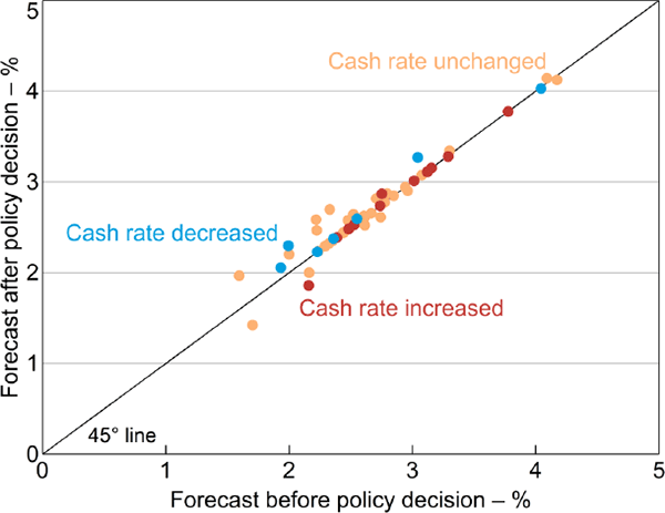
One potential issue with our baseline specification is that SMP forecasts are finalised after Board decisions are announced and thus incorporate financial market and other reactions to the announcement. This differs from the assumption made in Section 2 that the forecasts do not embody the current month's policy decision. This feedback makes analytical properties (such as our discussion of unbiasedness) complicated. However, Board decisions and market reactions to them usually have little effect on forecasts at the short forecast horizons we consider. This can be seen in Figure 3, which plots the Bank's official two-quarter-ahead inflation forecasts published several days after the Board meeting (y-axis) against the forecasts that were presented to the Board (x-axis).^[9] The latter are taken from the Bank's unpublished forecast archives and are only available from May 2001 onwards. The figure distinguishes between meetings where the cash rate was decreased (blue dots), increased (red dots) or left unchanged (orange dots). There is little evidence of feedback from the policy decision to the forecast. Although a handful of blue dots lie above the 45 degree line and a single red dot lies below the 45 degree line – suggesting a feedback effect – the magnitudes are trivial.^[10] The size of these feedback effects is likely to be much larger if we consider longer-run forecasts.

In Section 3 we consider some alternative specifications that make different timing assumptions about the forecasts. Robustness of our results to these variations supports our assessment that precise timing of the forecast does not matter much.

Concerns about potential feedback effects from the current month's policy decision – and the future path of policy rates – motivate us to use forecasts at fairly short horizons. Moreover, as Romer and Romer (2004) point out, both inflation and output growth are serially correlated enough that forecasts one and two quarters ahead provide a good indication of the likely forecasted path of the economy over longer horizons. Our decision to focus on short-horizon forecasts is also pragmatic, in that data on forecasts at longer horizons are often unavailable, particularly in the early part of our sample.

The results from estimating Equation (9) are presented in Table B1. The coefficients summarising the outlook for inflation (both the level of the forecast and the revision relative to the previous forecasting round) are jointly significant, with a p-value below 1 per cent. The Board reacts mainly to revisions to the inflation outlook. The sum of the two inflation terms is 0.19, such that a 1 percentage point increase in the two-quarter-ahead forecast for year-ended inflation leads to a 19 basis point increase in the cash rate. The small size of this response – which appears to imply that real interest rates decline in response to positive inflation surprises – is qualitatively similar (and in between) the estimates of Romer and Romer (2004) for the United States and Cloyne and Hürtgen (2016) for the United Kingdom. The coefficients on the output forecasts are positive but not statistically significant. Summing the two coefficients suggests that a 1 percentage point upgrade to the GDP growth forecast is associated with an increase in the cash rate of 6 basis points. The insignificance of the output forecasts may reflect that there is not enough independent variation in the output and inflation forecasts to disentangle their separate contributions.^[11]

The estimates suggest that the RBA clearly reacts to forecasts of inflation. As noted earlier, coupled with the substantial correlation between forecasts and future developments, this forward-looking behaviour implies a bias in estimates of the effects of policy on inflation in standard VAR models.

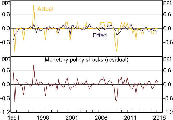
The top panel of Figure 4 shows the actual changes in the cash rate announced immediately after forecast-month Board meetings, along with the fitted values from Equation (9). The bottom panel of Figure 4 plots the residuals – our measure of monetary shocks. Some of the largest policy shocks occurred during the 2008–09 downturn, when the RBA cut the cash rate by more than historical relationships would suggest, given the forecasts for output and inflation generated at the time. In contrast, there were large contractionary shocks between August and December 1994, with the size of the monetary policy tightening appearing unusually large. As emphasised by Stevens (1999), this tightening cycle occurred at a time when the RBA had recently adopted inflation targeting and inflation expectations remained weakly anchored. In such an environment, a more aggressive response to anticipated inflation may be required to prevent the pick-up in inflation from occurring, as well as to reinforce credibility of the central bank's policy regime.

To be clear, Equation (9) is not intended as a full description of the Board's behaviour and we do not attempt to maximise its R². In particular, we intentionally do not control for other variables that the Board may consider when setting policy, such as the exchange rate and housing prices. It is possible that the Board responds to these variables above and beyond their direct impact on the forecasts for inflation and output. From the perspective of estimation, this would be desirable, since changes in the cash rate in response to variables such as housing prices provide us with the variation we require to estimate the effects of monetary policy on inflation and output.

2.2 Step #2: Effect of a Monetary Shock on Inflation and Output

2.2.1 Single-equation estimation

The simplest way to estimate the effect of a monetary policy shock on inflation is to regress the quarterly inflation rate on a constant, its own lagged values, and lagged values of our series of monetary policy shocks (an autoregressive distributed lag (ADL) model).

where π_t is trimmed mean inflation (measured in quarterly log differences, multiplied by 100) and S_t is our new measure of monetary shocks. We have assigned each policy shock to the quarter in which it occurs; for example, the estimated shock at the November 2008 Board meeting is the policy shock for 2008:Q4.

We can validly estimate using a single bivariate equation because we have already removed the effect of other influences on inflation through the forecast. This is in contrast to VAR identification strategies, in which the monetary shock is identified within the VAR itself. Following the literature, we assume that monetary policy does not affect inflation contemporaneously. This assumption does not affect our results. We include 8 lags of inflation and 12 lags of the monetary shock measure.^[12]

2.2.2 The inflation response

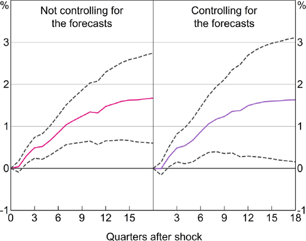
We first show a simple version of the price puzzle using an ADL model as a basis for comparison. The left panel of Figure 5 shows the dynamic response of the price level – that is, the cumulated response of quarterly inflation – to a 1 percentage point increase in interest rates. This is based on a version of Equation (9), in which we use changes in the cash rate announced at forecast-month Board meetings instead of our shock series. We find a price puzzle similar to those shown in Section 1.

The right panel of Figure 5 repeats this exercise using Equation (9). This differs from the left panel in that interest rate changes are purged of forward-looking behaviour using RBA forecasts. A contractionary shock to monetary policy is still estimated to have a positive and statistically significant effect on inflation and the price level. Purging the cash rate series of responses to the forecasts does not reduce the size of the price puzzle. This is the central result of our paper.

These results are surprising in several respects. The approach used to estimate Figure 5 is essentially the same as that of Romer and Romer (2004) and Cloyne and Hürtgen (2016). They find that purging policy of systematic responses to the forecast eliminates the price puzzle in the United States and United Kingdom, respectively. We do not see any obvious reason why results for Australia should be different. There are some differences in the nature of our data relative to that in the United States and United Kingdom, but sensitivity analysis in Section 3 does not indicate these differences are important. Conceptually, anticipatory policy is the obvious and standard explanation for the price puzzle and it is difficult to see how controlling for central bank forecasts would not remove this. We discuss these puzzles and some suggested solutions in Section 4.

The statistical significance of the price puzzle is also noteworthy, and has implications for the specification of our baseline. It implies that there is enough variation in our measure of policy shocks to permit confident inference. Were this not the case, there would be an argument for broadening our baseline measure of policy shocks to include other changes in interest rates, such as from months without recently updated forecasts or before the 1990s. We exclude these cash rate changes from our baseline – paying a cost in efficiency – because it is harder to confidently purge them of forward-looking behaviour. Nevertheless, as we show in Section 3, including these cash rate variations does not change our central results.

2.2.3 The output response

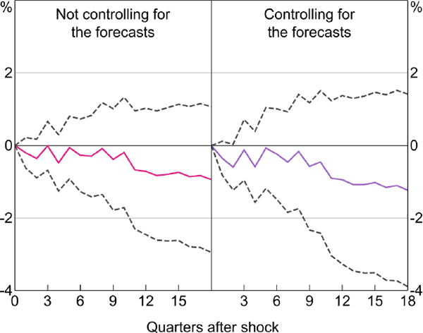
Given the implausible nature of our estimates for inflation, it is not clear what weight should be placed on our results for the effect of monetary policy on output. If we have failed to plausibly estimate the effect of monetary policy on inflation, it is hard to see how we can assume that the same approach and shock series will yield reliable estimates for the response of output. Nevertheless, policy multipliers for output are the focus of much of the literature. To estimate the impact of monetary shocks on output we simply replace the inflation terms in Equation (9) with quarterly real GDP growth. The left panel of Figure 6 shows the effect of a change in interest rates on real GDP. The right panel shows the effect of our shock series. Purging the interest rate series of anticipatory policy makes little difference to the results, again in contrast to the results of Romer and Romer (2004) and Cloyne and Hürtgen (2016) who find a larger effect on output when adjusting for anticipatory policy.

Footnotes

In other papers, Romer and Romer (2000, 2008) found the Federal Reserve's forecasts of inflation were a sufficient statistic for the inflation outlook, that is, other data (such as the forecasts of the private sector or the Federal Open Market Committee (FOMC)) do not provide useful additional information. [3]

The central bank also reacts to predicted inflation in the current quarter, but for simplicity we subsume this into the forecast. [4]

To see this,

View MathML

[5]

In addition to purging the policy rate of systematic responses to forecasts, Romer and Romer (2004) also use a historical narrative approach to remove movements in the actual federal funds rate (FFR) due to reasons unrelated to the stance of monetary policy. Such movements in the FFR are endogenous to economic conditions, and so using the actual FFR could lead to biased estimates of the effect of monetary policy on output and inflation. We do not need to create a series of intended policy changes, because over the sample period we consider (1990–2015), the target cash rate is the intended target policy rate. The RBA's domestic market operations have also ensured that the actual cash rate has remained close to the target rate (see Graph 1 in RBA (2015)). [6]

The Tulip and Wallace dataset does not contain inflation or GDP forecasts for 1991:Q3 or 1993:Q3. For these quarters, we interpolate forecasts using official forecasts from neighbouring quarters and Consensus forecasts for year-average growth in headline CPI and GDP. [7]

We also decide to include forecasts in year-ended percentage changes because that is how the forecasts are tabulated in the SMP and Board papers, and how they are presented to the RBA Board. Our archival forecast data do not contain quarter-on-quarter inflation forecasts prior to 2001. [8]

Where available, we use forecast data archived immediately before (or for the purpose of) the relevant Board meeting. If these forecasts are not available, we use the forecasts presented to the internal Policy Discussion Group, which is held on the Wednesday prior to the Board meeting, or to the Economic Group policy meeting. [9]

The few instances where the blue dots lie above the 45 degree line follow very large reductions in the cash rate, notably the 100 basis point cut in February 2009 and the 50 basis point cut in May 2012. [10]

When we omit the inflation forecasts from the model, the forecasts for output growth are jointly significant. In addition to multicollinearity, the insignificance of the GDP forecasts may be because the forecasts are not expressed in ‘gap’ terms; we find that replacing the GDP forecasts with forecasts for the unemployment rate leads to significant coefficient estimates (see Section 3). [11]

Romer and Romer (2004) estimate their ADL models using monthly data on industrial production and inflation. They use three years of lags for the policy shock in the output specification and four years in the inflation specification. We include three years of lags in both specifications, but our results are not affected by this decision. [12]