RDP 2017-02: Anticipatory Monetary Policy and the ‘Price Puzzle’ Appendix B: Additional Results
May 2017
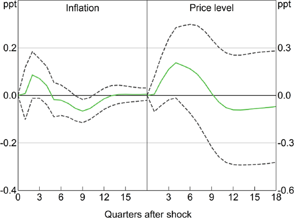
Figure B1: Effect of Monetary Policy on the Price Level –
FAVAR
Response to a temporary 1 percentage point shock

Notes: Price level is the cumulated response of underlying inflation; the IRFs are identified using a Cholesky decomposition with ordering: US GDP, commodity prices, GDP, underlying inflation, factor variable 1, factor variable 2, the cash rate, and the real TWI; confidence bands indicate 90 per cent intervals; sample period is 1990:Q2–2015:Q4
Sources: ABS; Authors' calculations
| Coefficient | Standard error | |
|---|---|---|
| Forecasts | ||
Underlying inflation  |
−0.05 | 0.05 |
Real GDP growth  |
0.05 | 0.03 |
| Change in forecasts relative to previous forecast round | ||
Underlying inflation  |
0.24*** | 0.08 |
Real GDP growth  |
0.01 | 0.05 |
Unemployment rate nowcast  |
0.00 | 0.01 |
| Cash rate prior to meeting (rm − 1) | 0.01 | 0.02 |
| Constant (α) | −0.10 | 0.19 |
|
Notes: Adjusted R2 = 0.20, Durbin-Watson = 1.90, No = 100; *, ** and *** indicate significance at the 10, 5 and 1 per cent level, respectively; Newey-West HAC standard errors Sources: ABS; Authors' calculations; RBA |
||