RDP 2016-10: The Effect of Consumer Sentiment on Consumption 4. Consumer Sentiment and Consumption
November 2016
- Download the Paper 1.39MB
In this section we investigate whether the sharp changes in sentiment between ALP and Liberal/National voters around changes of government affects consumption behaviour. We first investigate the response of individual-level spending intentions and then the response of postcode-level motor vehicle purchases. For each spending measure we first document the response around changes of government without the inclusion of controls. Treating the variation in sentiment that we exploit as a natural experiment, we do not need to include controls to provide valid identification. As a robustness test we also present results for each spending measure conditioning on available controls. At the individual level, the controls are the same variables used in Section 2. For the analysis of motor vehicle spending, we use the analogous set of postcode-level controls described in Section 3.2.3.
4.1 Spending Intentions
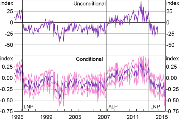
In the top panel of Figure 8 we show the difference in stated spending intentions between ALP and Liberal/National voters. Consumers report higher spending intentions when their political party holds government at the federal level, with statistical tests finding a break in the mean level of the series following an election that results in a change of government (see Table A1 for break test results).[9] This finding also carries through when we construct conditional spending intentions indices for ALP and Liberal/National voters using the methodology outlined in Section 2.3. The bottom panel of Figure 8 shows that differences in spending intentions between ALP and Liberal/National voters remain after controlling for an individual's economic and demographic characteristics.

Notes: Shows the effect of changes in government on spending intentions for a major household item; consumers were asked whether ‘now is a good time to buy a major household item’ and responses are either good, neutral, or bad; a separate index is constructed for ALP and Liberal/National voters as 100 plus the share of positive responses less the share of negative responses; top panel shows the difference between these two indices; bottom panel shows the conditional analogue; see notes to Figure 5
Sources: Authors' calculations; Westpac and Melbourne Institute
Comparing responses in the consumer sentiment survey to questions about economic conditions (Figure 3) and spending intentions (Figure 8) suggests a positive relationship between sentiment and spending intentions. Consumers report both a more positive economic outlook and positive spending intentions when their political party is in power. To formally test this, we estimate the following regression on the unit record consumer sentiment survey data:
where spendingi,t is the reported spending intention of individual i in month t and expecti,t is an individual's reported expectations of future economic conditions, Xi,j,t is the full set of economic and demographic control variables for person i listed in Section 2.3 and δt is a survey month dummy. The difficulty in estimating Equation (6) is that while expecti,t captures sentiment shocks, it also captures shocks to fundamentals factors that could jointly influence consumption and expectations. We therefore need an instrument that is correlated with the ‘sentiment’ but not the fundamental shock. Our instrument is an individual's partisanship. Specifically, we instrument expecti,t with a dummy variable that is equal to 1 if a survey respondent's voting intention matches the political party in office and is zero otherwise. As we have shown above, the sentiment of both ALP and Liberal/National voters move discretely and sharply in the month of an election where there is a change of government, with it being difficult to think of any current or past consumption fundamentals that could consistently increase sentiment by this amount in an election month.
We estimate Equation (6), with expecti,t instrumented by partisanship, over the period one year before and after an election with a change in government. We measure expecti,t using either of the two questions in the consumer sentiment survey asking individuals about their expectations of economic conditions over the next one and five years. These two questions relate to national economic conditions faced by all consumers and so abstract from considerations related to the distribution of government revenues. Note Equation (6) is estimated separately for expectations of economic conditions in one year's time and in five years' time. We code the answers to the spending intentions and expectations of future economic conditions questions as follows: positive responses take on a value of 3, unchanged or don't know responses take on a value of 2 and negative responses take on a value of 1. A linear probability model is estimated for both the first-stage and second-stage regressions.[10]
Results from three changes of government – 1996, 2007 and 2013 – are shown in Table 2. In the first stage, we find that consumers are more positive about future economic conditions when their partisanship matches that of the federal government. The precision of the first-stage results indicate that our instrument is strong.
For each change of government, we find that an improvement in expectations of future economic conditions has a statistically significant positive effect on spending intentions. This provides evidence that changes in sentiment can have a causal effect on stated spending intentions at the individual consumer level.
Second stage:  |
||||||
|---|---|---|---|---|---|---|
| 1996 election | 2007 election | 2013 election | ||||
| expect: next year | 0.360*** (0.031) |
0.302*** (0.061) |
0.435*** (0.061) |
|||
| expect: 5 years | 0.524*** (0.047) |
0.329*** (0.062) |
0.511*** (0.077) |
|||
| Controls | Yes | Yes | Yes | Yes | Yes | Yes |
| Observations | 22,650 | 21,954 | 24,985 | 24,045 | 26,241 | 26,000 |
First stage:  |
||||||
| 1996 election | 2007 election | 2013 election | ||||
| expect: next years | expect: 5 years | expect: next years | expect: 5 years | expect: next years | expect: 5 years | |
| support | 0.437*** (0.013) |
0.307*** (0.014) |
0.237*** (0.013) |
0.242*** (0.014) |
0.304*** (0.017) |
0.252*** (0.016) |
| Controls | Yes | Yes | Yes | Yes | Yes | Yes |
| Observations | 22,650 | 21,954 | 24,985 | 24,045 | 26,241 | 26,000 |
|
Notes: Each regression uses individual response data pooled over the period one year before and after each election with a change in government: March 1996, November 2007 and September 2013; the variable expect: next year is beliefs about the ‘expected change in general economic conditions over the next year’, with responses coded as 1 (negative), 2 (unchanged/don't know), and 3 (positive); expect: 5 years is responses to the analogous question about economic conditions over the next five years; support takes the value unity if a survey respondent's self-identified voting intention matches the political party in office and zero otherwise; spend is responses to the question ‘do you think now is a good time to buy a major household item’ with responses coded as 1 (bad time), 2 (neither good/nor bad), and 3 (good time); the set of controls Xi,j,t includes: gender, age, occupation, education, home ownership, income, metro/non-metro, plus a constant; δt is a survey/month fixed effect; the categorical variables expect and spend are treated as linear variables; the first stage is estimated using OLS and the second stage is estimated using two-stage least squares; robust standard errors have been used and are reported in parentheses; ***, ** and * denote results statistically different from zero at the 1, 5 and 10 per cent levels, respectively |
||||||
4.2 Actual Spending Data
We now investigate whether the stated spending intentions data are consistent with the postcode-level motor vehicle purchases data.
4.2.1 Without controls
We would like to know if differences in self-reported spending intentions between ALP and Liberal/National voters are reflected in differences in observed motor vehicle sales. ALP voters became substantially more optimistic about economic conditions than Liberal/National voters when the ALP won government at the 2007 election. If the opinions expressed in the sentiment survey are indicative of actual consumption behaviour we would expect to see a relative increase in motor vehicle sales in ALP-leaning postcodes. Conversely, we would expect to see a relative increase in motor vehicle sales in Liberal/National-leaning postcodes following the 2013 election when the Liberals/Nationals won government.
To see if self-reported spending intentions are informative about actual consumption, we estimate the following regression over the period 2004–14:
where mvit is per capita motor vehicle sales in postcode i in quarter t, αi is a postcode-specific fixed effect, dt is an indicator variable taking the value unity in period t and zero otherwise, ALPτ is the ALP vote share in postcode i for an election held at time τ, and εi,t is an error term.[11] The coefficients δj are quarterly fixed effects, capturing all variation in motor vehicle sales that is common across postcodes, such as seasonality, changes in motor vehicle prices, and aggregate economic shocks. The coefficients of interest are βj, indicating the relationship in quarter t between ALP vote share and per capita motor vehicle sales. The omitted category in the regression is the quarter in which the election is held, so all estimated βj coefficients are relative to that period. We estimate Equation (7) separately for the 2007 and 2013 elections using weighted least squares, with weights equal to the average number of motor vehicle sales over the two years prior to the change in government under consideration at time τ.[12] We are primarily interested in the change in βj coefficients around the 2007 and 2013 changes of government, but report coefficient estimates for the entire sample period 2004–14. The most relevant estimates of Equation (7) are those based on weights closest to the change of government under consideration. Standard errors are clustered at an electorate level.
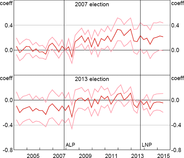
The top panel of Figure 9 presents the βj coefficient estimates from Equation (7) together with two standard error confidence bands, using vote shares for the 2007 Federal election. The coefficient estimates indicate the log change in the quarterly level of motor vehicle sales, relative to the December quarter 2007, when moving from a hypothetical postcode with only Liberal/National voters to one with only ALP voters. Shortly after the ALP won government at the 2007 Federal election, there was a sustained increase in the level of motor vehicle sales in ALP-leaning postcodes relative to Liberal/National-leaning postcodes. In the three years following the 2007 election, the βj coefficients average to about 0.1. This indicates that going from a postcode with no ALP voters to a postcode where everyone votes for the ALP increases per capita motor vehicle sales by 10 per cent. The estimated βj coefficients over this period are for the most part statistically significant. The largest difference in the average level of motor vehicle sales between ALP and Liberal/National postcodes occurred around 2012. This lines up with the largest difference between ALP and Liberal/National voters in spending intentions for a major household item from the consumer sentiment survey.

Notes: Top panel shows coefficient estimates βj for Equation (7) using vote share data from the 2007 Federal election, the omitted category is the December quarter 2007 when the ALP won government; bottom panel shows coefficient estimates βj using vote share data from the 2013 Federal election, the omitted category is the September quarter 2013 when the Liberal/National party won government; standard errors are clustered by federal electorates; vertical lines show dates when government changed hands
Sources: ABS; Authors' calculations; VFACTS
The bottom panel of Figure 9 reports analogous results using vote share data from the 2013 election when the Liberal/National party won office. While the fall in the estimated βj coefficients start prior to the 2013 election, consistent with the spending intentions data, an average of the βj coefficients indicates a 7 percentage point lower level of motor vehicle purchases by ALP voters relative to Liberal/National voters in the two years after the ALP's loss of government compared to the ALP's last two years in office.
The results in this section indicate that differences in consumer sentiment between ALP and Liberal/National voters are reflected in differences in motor vehicle sales, providing some validation for information contained in the sentiment survey. Further, the results, particularly from the 2007 election, indicate that consumer sentiment can contain forward-looking information about consumption, given that sentiment changes precede consumption changes.
4.2.2 With controls
Partisanship is correlated with a range of economic indicators (Table 1). An incoming government could enact tax and transfer policies that favour its supporters. This can have a direct effect on consumption by changing the distribution of income, implying that government policy, rather than sentiment, could be responsible for the changes in motor vehicle consumption described in the previous sub-section. As noted before, policy set by the federal government cannot be targeted to specific individuals, but rather to particular groups of people. While our identification approach uses partisanship as a source of variation in economic perceptions, there would ideally also be no difference in how government policy affects ALP and Liberal/National voters. We use two approaches to control for these differences. In the first approach, we try and construct a measure of pure partisanship by isolating variation in the ALP vote share at each change of government that is uncorrelated with observable economic differences between ALP and Liberal/National voters. We then use this variation as our source of identification. We also employ difference-indifference regressions, which allow us to control for differences in income growth across postcodes.
4.2.2.1 Pure partisanship
To construct a measure of pure partisanship, we separately regress the ALP vote share at the 2007 and 2013 elections on a wide range of economic variables and take the residual series. The regression includes the full set of demographic and industry variables reported in Table 1, as well as controls for the geographic characteristics of a postcode. (Regression results are reported in Table A2.[13]) The economic control variables absorb between 55 and 60 per cent of the postcode-level variation in vote shares.
We then re-estimate Equation (7), replacing the observed ALP vote share variable with our measure of pure partisanship. Formally, we estimate the regression
where  is the residual for postcode i from a
regression of the ALP vote share for the election held at date τ on the set of
control variables described above. To allow for the use of a generated regressor, standard
errors are constructed using 1,000 bootstrap replications, with resampling conducted at the
electorate level.
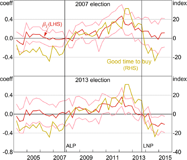
Results using this residual variation in the ALP vote share for both the 2007 and 2013 elections show a qualitatively similar profile to that from Equation (7) without controls (compare Figures 9 and 10). We again find little evidence of a pre-trend before the 2007 election. Following the ALP's victory at the 2007 election we estimate that a positive ALP vote share residual is associated with a higher level of motor vehicle purchases. Also consistent with the consumer sentiment survey, this pattern reverses around the time of the 2013 election, at which the Liberal/National party formed government. The change in motor vehicle purchases is more pronounced than in the regression without controls. Although the downward trend in motor vehicle purchases began about 18 months prior to the 2013 election, it does line up with the timing of the downward trend in the difference between ALP and Liberal/National voters on whether it is a good time to buy a major household item in the consumer sentiment survey, which is also plotted in Figure 10.

Notes: Shows coefficient estimates βj for Equation (8); top panel shows coefficient estimates βj using vote share data from the 2007 Federal election, the omitted category is the December quarter 2007 when the ALP won government; bottom panel shows the coefficient estimates βj using vote share data from the 2013 Federal election, the omitted category is the September quarter 2013 when the Liberal/National party won government; lighter lines are 95 per cent confidence bands calculated from 1,000 bootstrap replications; resampling was conducted at the federal electorate level; ‘Good time to buy’ is the difference between ALP and Liberal/National voters in self-reported spending intentions for a major household item; vertical lines show dates when government changed hands
Sources: ABS; Authors' calculations; VFACTS; Westpac and Melbourne Institute
Because the control variables absorb over half the variation in the ALP vote share across postcodes, the standard errors around our estimates are now larger. But we nonetheless believe that the point estimates are informative, particularly given that they follow a broadly similar pattern to the point estimates from the regression without controls. These results provide further evidence that consumers' stated spending intentions in the sentiment survey do correspond with observed behaviour. Given our extensive use of controls, these results also provide further evidence that changes in sentiment have a causal effect on consumption.
4.2.2.2 Difference-in-difference regressions
We have investigated whether the differential consumption response of Liberal/National and ALP voters around changes of government can be explained by differences in observable economics characteristics. We relied on point-in-time data, mostly from the 2006 and 2011 Census. This approach controls for differential income shocks correlated with observable economic characteristics. To allow for differential income shocks not correlated with observable economic characteristics, we now adopt a difference-in-difference framework, which allows us to control for changes in postcode-level incomes over time. Here we argue that if different groups of voters experience different shocks then this should show up in their incomes.
We estimate the following difference-in-difference regression at an annual frequency:
where Δhlog(mvi,t+h) is the percentage change in per capita motor vehicle purchases in postcode i between 2007 and year 2007 + h, where h = {1,2,…,6}. Control variables include postcode-level growth in taxable income, Δhlog(inci,t+h), and the full set of control variables Xi,j,h listed in Table 1. Because Australian Taxation Office income data are available for only one year after the 2013 election we only estimate Equation (9) for the 2007 election. As before, we use the average number of motor vehicle purchases over the two years before the 2007 election as regression weights.
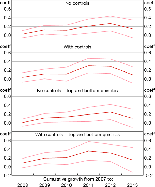
We estimate Equation (9) separately over six different time horizons: 2007 to 2008 (h = 1), 2007 to 2009 (h = 2), and so on, until the period 2007 to 2013 (h = 6). Figure 11 shows estimates of βh in the presence and absence of the control variables. Figure 11 can be interpreted as follows: the first data point at 2008 shows the effect on growth in motor vehicle sales from 2007 to 2008 when moving from a postcode with no ALP voters to one with only ALP voters. The second data point for 2009 shows this same effect, but for motor vehicle sales over a two year window from 2007 to 2009, and so on. The size of these estimated effects are non-trivial: going from a hypothetical postcode with only Liberal/National voters to another postcode with only ALP voters is estimated to have increased per capita motor vehicle purchases by around 30 per cent four years after the 2007 election, even after we control for changes in income.
For postcodes with a similar proportion of ALP and Liberal/National voters, changes of government have relatively little net effect on sentiment, suggesting that much of our identification comes from postcodes at the political ‘extremes’. Reflecting this, the results are similar if we restrict the estimation sample to postcodes in the top and bottom quintiles of ALP vote share at the 2007 Federal election.
Overall, the estimates presented in this sub-section are consistent with our earlier results, providing further evidence that sentiment has a causal effect on consumption. Again, we find evidence that consumer sentiment contains forward-looking information, as changes in sentiment occur before changes in consumption.

Notes: Shows coefficient estimates βh for Equation (9); each coefficient βh is from a separate regression; top panel shows coefficient estimates βh from a regression including no controls; the second panel includes the full set of controls listed in Table 1; the third and bottom panels repeat the first two panels, restricting the data sample to postcodes in the top and bottom population-weighted quintiles of ALP vote share at the 2007 Federal election; the lighter lines are two standard error bands
Sources: ABS; Authors' calculations; VFACTS
Footnotes
The 1996 election was held on 2 March. The consumer sentiment survey is conducted at the end of each month and can continue into the start of the following month. This is why the break in the spending intentions series for the 1996 election occurs in February 1996. [9]
Both the spending intentions and sentiment data are categorical. We choose to estimate the first-stage equation using a linear probability model, rather than an ordered probit, because with instrumental variables, OLS estimates of the first stage produce consistent estimates. First-stage estimates using a probit model are consistent only under restrictive assumptions. We also estimated the second stage using a probit model and the first stage as a linear probability model. The results were similar to that in the text. [10]
The use of a log transformation for the dependent variable results in the exclusion of observations with zero motor vehicle sales in a given quarter. Based on the regression weights, which are equal to the average number of motor vehicle sales over the two years prior to a change of government, the postcodes that contain a zero observation in any given quarter account for less than 1.5 per cent of motor vehicle sales over the weighting period. As an alternative, we have estimated Equation (7) with the level of per capita motor vehicle sales as the dependent variable, which does not result in the exclusion of any data. The results are very similar, and so we present results using the log transformation to facilitate interpretation of our results. [11]
Using population weights instead does not materially change our results. [12]
For the 2007 election, we use 2006/07 mean taxable income, and for the 2013 election we use 2012/13 data. [13]


