RDP 2016-10: The Effect of Consumer Sentiment on Consumption Appendix A: Reconciliation with Mian et al (2015)
November 2016
- Download the Paper 1.39MB
Our paper is most closely related to Mian et al (2015). They use US data to investigate whether changes in county-level consumption following a change in the party occupying the US presidency are related to county-level voting outcomes. While we find that an increase in sentiment leads to higher consumer spending, they find no statistically significant relationship between sentiment regarding government economic policy and consumer spending. We offer a few explanations as to why our results differ to theirs.
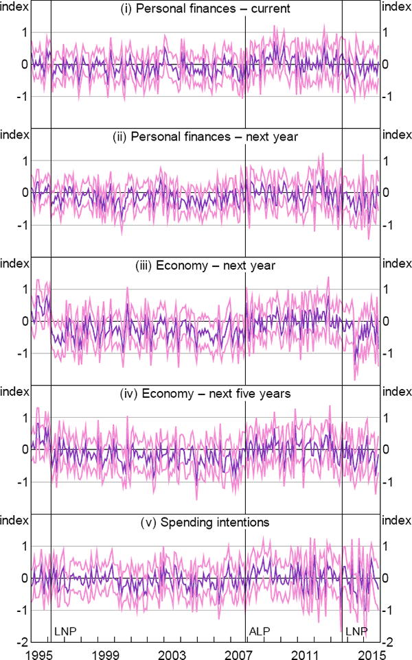
Firstly, the Australian consumer sentiment survey asks respondents about their voting intentions. In contrast, Mian et al have to impute an individual's partisanship based on the county where they live. To see the effect of imputing partisanship, using our data we impute an individual's partisanship based on their postcode. In particular, we re-compute conditional consumer sentiment indices using the same methodology outlined in Section 2.3, but instead of using an individual's self-reported voting intention we use the postcode-level ALP vote share in their postcode of residence at the 2007 election. Comparing the results in Figure A1 where partisanship is imputed to that in Figure 3 of our paper, where we observe partisanship, we can see that imputing partisanship introduces noise into the data. Nonetheless, these estimates do suggest that ALP voters are more pessimistic about the national economy (sub-indices (iii) and (iv) in Figure A1) when the Liberal/National party is in government. But the effect of partisanship on spending intentions is too small to detect when voting intention is imputed from postcode-level vote shares. These results using the imputed measure of partisanship mirror the findings of Mian et al for the United States, and so provide a reconciliation between our findings.

Notes: Estimates repeat those of Figures 5 and 8 using imputed rather than self-reported partisanship as the dependent variable; the measure of partisanship is the ALP vote share at the 2007 Federal election in the postcode of residence for each survey respondent; see notes to Figures 5 and 8
Sources: Authors' calculations; Westpac and Melbourne Institute
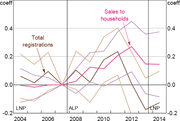
In terms of how motor vehicles are measured, because we are interested in the effect of consumer sentiment on household consumption, we use motor vehicle sales to households. Mian et al (2015) use registration data which includes motor vehicle sales to businesses and governments in addition to households. To see the effect of using total motor vehicle sales data we re-estimate Equation (7) from our paper using Australian motor vehicle registration data. The data are sourced from the Australian Bureau of Statistics and are available on an annual basis. Figure A2 shows the effect of an increase in the ALP vote share on motor vehicle sales. As the figure indicates, the standard errors are larger when we use registration data rather than just sales to households. It also now becomes unclear whether changes in sentiment affect consumption, with the estimated coefficients having a saw-toothed pattern around the 2007 election.[15]
Finally, voting in Australia is compulsory. In contrast, voting in the United States is voluntary. This can lead to selection issues. For example, it is well known that voter turnout can be affected by opinion polls. This leads to measurement error which can downwardly bias the estimated effect of partisanship on consumption.

Notes: Shows coefficient estimates βj for Equation (7), using annual vehicles data and vote share data from the 2007 Federal election; the coefficient estimates βj are relative to the omitted year 2007, when the ALP won government; we measure per capita motor vehicle purchases in two ways: from sales to households and from registration data that includes sales to households, businesses and government; registration data are available only at an annual frequency; the lighter lines are 95 per cent confidence bands; vertical lines show dates when government changed hands
Sources: ABS; Authors' calculations; VFACTS
| Double maximum test | Information criteria | SupF test | Sequential test | Break dates | Changes of government | ||
|---|---|---|---|---|---|---|---|
| 3 breaks | 4 breaks | 5 breaks | |||||
| UD-Max | BIC | SupF(2|1) | 4 breaks | Feb 1996 | Feb 1996 | Feb 1996 | Mar 1996 |
| 81.08*** | 5 breaks | 113.80*** | Mar 2008 | Dec 2007 | Jun 2000 | Nov 2007 | |
| WD-Max | LWZ | SupF(3|2) | Oct 2013 | Apr 2010 | Dec 2007 | Sep 2013 | |
| 81.08*** | 4 breaks | 74.53*** | Sep 2013 | Apr 2010 | |||
| SupF(4|3) | Sep 2013 | ||||||
| 33.62*** | |||||||
| SupF(5|4) | |||||||
| 5.16 | |||||||
|
Notes: Reports tests for a break in the difference between the mean level of spending intentions for ALP and Liberal/National voters; the double maximum tests are for an unspecified number of breaks against the null of zero breaks; both the UD-Max and WD-Max test statistics evaluate an F-statistic for 1–5 breaks, with the break points selected by global minimisation of the sum of squared residuals; the UD-Max statistic weights the five F-statistics equally, while the WD-Max statistic weights the F-statistics such that the marginal p-values are equal across the number of breaks; the WD-Max test statistic reported is for a 1 per cent significance level test; the LWZ statistic is a modified Schwarz criterion; the SupF(i + 1|i) test is for i + 1 breaks against the null of i breaks; the sequential test selects the number of breaks stepwise from zero breaks using the SupF test assuming a 5 per cent significance level; the break dates are those identified by minimising the sum of squared errors conditional on the number of breaks; ***, ** and * indicate results statistically different from zero at the 1, 5 and 10 per cent levels, respectively |
|||||||
| 2007 election | 2013 election | |
|---|---|---|
| Log taxable income | −19.22*** (4.68) |
−24.32*** (5.04) |
| Average age (yrs) |
−0.20* (0.11) |
−0.24** (0.12) |
| Share with Bachelor's degree or higher | 1.17*** (0.22) |
1.12*** (0.20) |
| Share who rent | 0.00 (0.05) |
−0.02 (0.06) |
| Unemployment rate | 1.73*** (0.21) |
1.05*** (0.25) |
| Share in white-collar profession | −0.80*** (0.16) |
−0.74*** (0.19) |
| Industry share of employment: | ||
| Agriculture | −0.64*** (0.14) |
−0.71*** (0.13) |
| Mining and construction | −0.39*** (0.15) |
−0.36*** (0.14) |
| Manufacturing | −0.16 (0.13) |
0.23 (0.16) |
| Retail and wholesale trade | −0.92*** (0.17) |
−1.13*** (0.20) |
| Services | −0.39** (0.19) |
−0.53*** (0.19) |
| Health and education | −0.60*** (0.16) |
−0.42** (0.17) |
| Arts and accommodation | −0.75*** (0.25) |
−0.54** (0.24) |
| Other | −1.16** (0.52) |
−1.37*** (0.48) |
| Region: | ||
| Inner regional | −4.82*** (1.45) |
−5.02*** (1.56) |
| Outer regional | −5.16*** (1.77) |
−5.91*** (1.75) |
| Remote | −2.00 (2.50) |
−3.36 (2.50) |
| Very remote | 1.87 (3.75) |
1.15 (3.87) |
| R2 | 0.61 | 0.55 |
| Observations | 2,265 | 2,264 |
|
Notes: Reports coefficient estimates from a regression of the ALP vote share on postcode-level characteristics; for the 2007 Federal election, income is measured using 2006/07 taxable income data and other variables are taken from the 2006 Census; for the 2013 Federal election, income is measured using 2012/13 taxable income data and other variables are taken from the 2011 Census; observations are weighted by the number of voters in a postcode at each election; baseline covariates are: home owner, blue-collar profession, public sector industry, and metropolitan location; postcodes in the ACT are excluded; robust standard errors have been used and are reported in parentheses; ***, **, and * denote results statistically different from zero at the 1, 5 and 10 per cent levels, respectively |
||
Footnote
Mian et al also use credit card data in their analysis. Unfortunately we do not have access to credit card data. [15]