RDP 2016-06: Jobs or Hours? Cyclical Labour Market Adjustment in Australia Appendix A: Decomposing the Cyclical Adjustment of Total Hours
September 2016
- Download the Paper 1,085KB
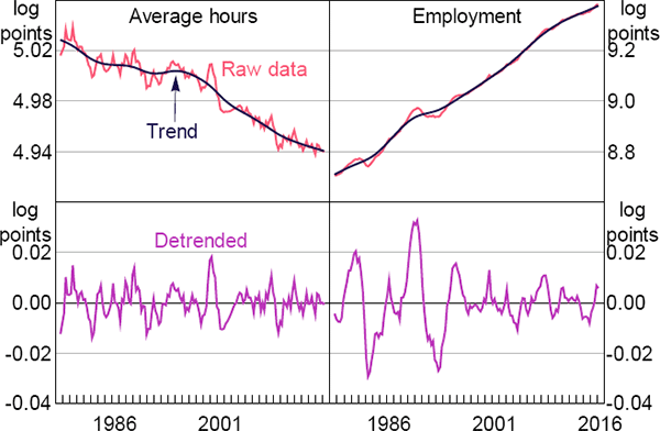
Data for total hours worked, employment, average hours worked and real GDP in Sections 2 and 3.3 are in logs and individually detrended using a HP filter with smoothing parameter λ = 1,600. The top panel of Figure A1 shows the raw data (in logs) and the HP trend of each series, while the bottom panel shows the detrended version of each series.

Notes: Trend is HP filter with smoothing parameter λ = 1,600; detrended series are the difference between the raw data series and trend
Sources: ABS; Authors' calculations
The estimates in Table 1 are based on the decomposition outlined in Merkl and Wesselbaum (2011). The contribution of average hours to cyclical adjustment in total hours is given by
where tothrst and avhrst are total hours worked and average hours worked, respectively. The estimate gives the proportion of variation in total hours that derives from average hours, both directly and indirectly through its correlation with employment. Similarly, the contribution of employment to cyclical adjustment in total hours is given by
where empt is employment. These estimates are equivalent to the slope coefficients in simple ordinary least squares regressions of average hours on total hours and employment on total hours, respectively.
Using alternative methods to detrend the data does not affect the main conclusions (Table A1). Using four-quarter-ended log differences rather than the HP filter does not have a material effect on the results. Using one-quarter-ended log differences suggests a larger role for average hours adjustments prior to 1998 relative to the other detrending methods, although this is likely to reflect the high quarter-to-quarter volatility in the average hours data.
The regression framework also allows us to perform the Quandt-Andrews structural break test for an unknown break point. This test suggests that the break in the coefficient on total hours worked (in either the average hours or employment specification) in 1998:Q2 is significant at the 1 per cent level. The test is for a break in the coefficient in the regression equation, although also allowing for a break in the constant does not change the result. We also tested the robustness of this break date using alternative detrending methods based on a Chow test with the break date set to 1998:Q2. There was evidence of a statistically significant break in 1998:Q2 using one-quarter-ended or four-quarter-ended log differences, rather than the HP filter.
| Full sample | 1978–98 | 1998–2016 | |
|---|---|---|---|
| HP filter (λ = 1,600) | |||
| Employment, θE | 73 | 80 | 42 |
| Average hours, θA | 27 | 20 | 58 |
| Log differences (four-quarter-ended) | |||
| Employment | 70 | 79 | 45 |
| Average hours | 30 | 21 | 55 |
| Log differences (one-quarter-ended) | |||
| Employment | 51 | 57 | 40 |
| Average hours | 49 | 43 | 60 |
Notes: In both the HP filter and the two-stage least square specifications, all variables are in logs and detrended with an HP filter (λ = 1,600); for a definition of ‘downturn periods’, see footnote 5 Sources: ABS; Authors' calculations |
|||

