Bulletin – September 2014 Australian Economy Unemployment and Spare Capacity in the Labour Market
- Download the article 456KB
Abstract
The unemployment rate provides an important gauge of spare capacity in the labour market and the economy more generally. However, other factors also affect unemployment, which complicates its interpretation when informing monetary policy. Statistical methods can be used to estimate the extent to which the unemployment rate reflects spare capacity versus more enduring structural factors. This involves estimating the NAIRU. Information can also be gleaned from the composition of unemployment, as jobseekers with certain characteristics may be more indicative of spare capacity than others. These approaches suggest that spare capacity in the labour market has increased over the past few years but remains well below that which prevailed over much of the 1990s.
Introduction
An important consideration for monetary policy is the extent of spare capacity in the economy. This depends on the balance of demand for goods and services relative to the economy's potential to produce them. A shortfall of demand results in spare capacity and places downward pressure on inflation, while an excess of demand results in capacity becoming constrained, placing upward pressure on inflation.
A key indicator of spare capacity in the economy is the unemployment rate. A high unemployment rate means that there is a large pool of workers willing to work but not engaged in production, suggesting that the economy is operating below its potential. However, there are other reasons why someone may be unemployed, meaning that some individuals will be looking for work even when an economy is producing at its potential; for example, some people that wish to change jobs may spend time searching for the right role. The rate of unemployment that is consistent with the economy producing near its potential will be that associated with a stable rate of inflation, so it is known as the ‘non-accelerating inflation rate of unemployment’ (NAIRU). When unemployment deviates from this level, it suggests that the economy is producing above or below its prevailing potential.
It is difficult to know whether a change in the unemployment rate indicates a change in spare capacity, or whether it instead is due to a change in the NAIRU. This article investigates the drivers of unemployment and its relationship with spare capacity in the labour market. The following section expands on the factors that explain the existence of unemployment. Two approaches for extracting information about the extent of spare capacity reflected in unemployment are then examined. The first approach uses information on inflation in wages and prices to infer both the portion of the unemployment rate that is spare capacity and the portion that is the NAIRU. The second approach looks at whether some types of unemployment have more bearing on inflation than others.
The Causes of Unemployment
Each month, the Australian Bureau of Statistics (ABS) samples about 50,000 individuals to assess their labour force status. Individuals that have worked one hour or more in the survey's reference week are classified as ‘employed’. Those that are not employed, but are actively searching for work and available to start, are classified as ‘unemployed’. The remainder are considered to be outside the labour force.
The level of unemployment is affected by the balance of flows into and out of unemployment (Figure 1). Individuals enter unemployment when they are ‘separated’ from a job, because they are retrenched or resign. In turn, individuals exit unemployment when they are successful in finding a job – that is, they are ‘matched’ with a vacancy. There are also flows between unemployment and outside the labour force, such as individuals that start or stop searching for work. Each month, flows into and out of unemployment are very large; nearly half of the pool of unemployed leaves unemployment, either finding a job or moving out of the labour force, while a similar number of new individuals enter unemployment.
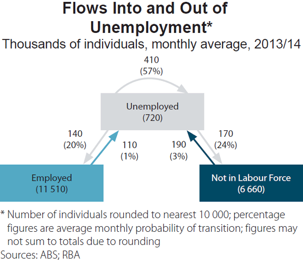
The figure shows the average monthly flows between the pools of unemployed workers, employed workers and those not in the labour force over the financial year 2013/14. Of the 710,000 unemployed workers, a little over one half remain unemployed each month. Around one quarter of unemployed workers exit the labour force each month, while a similar number enter unemployment from outside the labour force. A little under one quarter of unemployed workers find work each month, while a similar number of employed workers enter unemployment.
These flows provide the basis for understanding the causes of unemployment. In principle, there are three causes of unemployment. In practice, these causes cannot be measured directly, and the margins between them may be blurred, but they provide a useful framework for thinking about unemployment:
- Frictional unemployment results from the regular movement of individuals in the labour market. The labour market is very dynamic; each year, around one million workers, or roughly 1 in 12, change jobs (D'Arcy et al 2012). In addition, many individuals transition into and out of the labour force according to their personal circumstances. This movement of workers is beneficial, as it facilitates the efficient allocation of labour across the economy. However, the labour market is characterised by a large degree of diversity – both in terms of workers and jobs. This means that workers must invest time and effort in searching for the right job, and firms do likewise in looking for suitable candidates. As a result, individuals are not matched immediately with vacant jobs and may experience a temporary period of unemployment.
- Structural unemployment results from a more fundamental mismatch between jobs and workers. For example, when the economy undergoes structural change, the industrial structure of activity evolves, the types of jobs change as technology advances, and the location of jobs also shifts. These changes can produce a more enduring mismatch between unemployed workers and available jobs, reducing the ‘efficiency’ with which they are matched and increasing unemployment. Those individuals with skills in declining industries may have little chance of finding work until they develop new skills or move to a region with better opportunities. Although the economy is always undergoing change, structural unemployment may tend to be higher in periods when such change is more substantial.[1]
- Cyclical unemployment is the result of changes in aggregate conditions in the economy over the course of the business cycle. A shortfall of demand in the economy will result in a lack of jobs relative to the number of people that want to work. Both flows into and out of unemployment will be affected as demand fluctuates over the business cycle. Firms experiencing weaker demand for the goods and services they produce will reduce the amount of labour they employ, laying off existing workers and hiring fewer new workers. As a result, involuntary flows into unemployment will rise while the unemployed will experience a lower probability of finding work. The opposite will occur when demand strengthens; firms will look to expand their operations by hiring new workers and retaining existing staff, lowering unemployment and absorbing spare capacity in the labour market.
These classes of unemployment are not independent of each other. For example, a period of high cyclical unemployment might lift structural unemployment for a while – a phenomenon known as hysteresis. This occurs when individuals are unemployed for a long period of time and suffer lasting damage to their job prospects, reducing their probability of being matched to a vacant job. In particular, workers that have been unemployed for longer might see a deterioration of their skills and productivity (Pissarides 1992; Ljungqvist and Sargent 1998) or be regarded as less employable, reducing their chances of finding employment further (Blanchard and Diamond 1994).
Of the three causes of unemployment, cyclical unemployment is the real source of spare capacity in the sense that it indicates that the economy is producing below its potential. In contrast, frictional and structural unemployment do not represent unemployed persons who could easily be pulled into employment if demand was higher. These classes of unemployment exist even when labour markets are in equilibrium, such that an increase in labour demand would not reduce this type of unemployment.[2] Instead, these types of unemployment are largely tied to the process of productive resources (labour) moving around the economy and into and out of the labour force. While these other causes of unemployment do have social costs, detracting from households' incomes and welfare, they are best addressed with policies that focus on the supply side of the labour market, rather than by stimulating aggregate demand.
While unemployment is a useful measure of spare capacity, it does not capture all aspects of capacity utilisation in the labour market. Firms that are seeking to reduce their labour market input can adjust the hours worked by existing staff (resulting in ‘underemployment’), and some individuals out of work may become discouraged and stop searching for a job (resulting in ‘marginal attachment’ to the labour force). These are important issues, but they are beyond the scope of this article.[3]
Spare Capacity, Inflation and the NAIRU
The extent of any spare capacity in the economy exerts an influence on prices and wages. Excess capacity in the market for goods and services will place downward pressure on inflation in their prices. Similarly, spare capacity in the labour market will place downward pressure on the growth of wages.[4] Conversely, an excess of demand in the economy will result in faster inflation in both wages and prices. Therefore, to the extent that the unemployment rate is a useful measure of spare capacity, it should have an inverse relationship with inflation in both wages and prices. This inverse relationship is known as the Phillips curve, and can be seen in Australian data for the past two decades. Periods with higher unemployment rates have tended to be associated with slower inflation in both wages and prices (Graph 1).
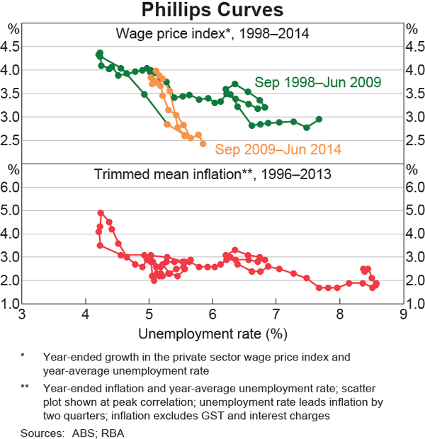
In principle at least, frictional and structural unemployment should not influence the course of prices or wages. Hence, these types of unemployment should be captured by the NAIRU – the level of unemployment that causes neither an increase nor decrease in inflation. While it is not possible to observe the NAIRU directly, it can be inferred from the position of the Phillips curve. For example, there is evidence that the NAIRU has fallen over the past 15 years because the basic Phillips curves for wages and prices have shifted to the left.[5] In recent years, an unemployment rate of around 5½–6 per cent has seen slow wages growth, well below 3 per cent per annum. However, in the late 1990s, much higher rates of unemployment of almost 8 per cent did not see such slow growth in wages. This suggests that factors other than spare capacity were responsible for the higher unemployment rate at that time, meaning that the NAIRU is likely to have been higher.
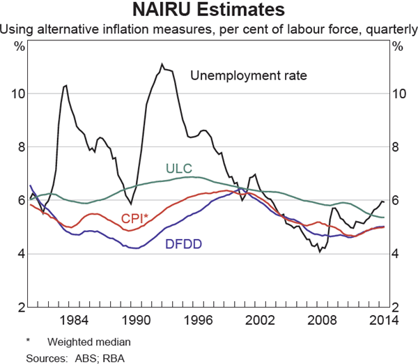
Estimates of the NAIRU can be obtained with statistical models. Specifically, a Phillips curve is estimated as a function of two unobserved terms: the component of unemployment that does not affect inflation, the NAIRU, and the component that captures economic slack and, hence, does affect inflation. The particular model used here is set out in Gruen, Pagan and Thompson (1999), and the results are an update of their findings (for further details, see Appendix A). Three different estimates of the NAIRU are produced using different measures of inflation: underlying inflation as measured by the weighted median measure of inflation in the consumer price index (CPI); inflation based on the national accounts domestic final demand deflator (DFDD); and inflation of labour costs based on the national accounts measure of unit labour costs (ULC). The three NAIRU estimates have deviated substantially in some periods (Graph 2). A positive gap between the actual unemployment rate and the estimate of the NAIRU indicates evidence of spare capacity in the labour market, and vice versa.
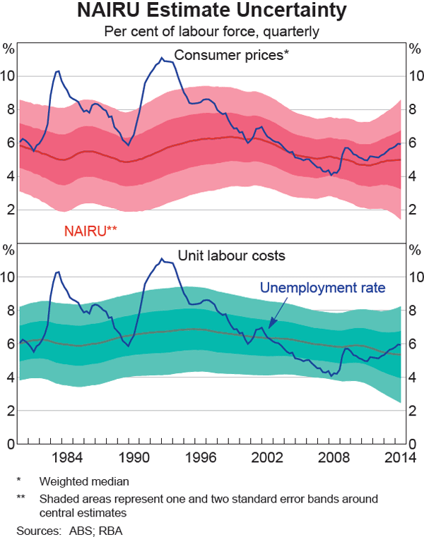
There are various conceptual and empirical reasons to be cautious about estimates of the NAIRU.[6] First, the figures are central estimates from a model and have wide confidence bands around them (Graph 3). These estimates are sensitive to the length of the period over which they are estimated. The estimates often also change as more data come to hand, with the profile toward the end of the sample period particularly prone to revision. This end-point problem detracts from the ability to use these estimates in real time. Finally, the estimates also rely on having a ‘correct’ model of inflation. If the model fails to control correctly for the factors that are important to inflation, or if the nature of the inflation process changes over time, then the estimates will not be accurate. Indeed, different specifications of the Phillips curve model can generate quite different estimates of the NAIRU.
The Observable Characteristics of the Unemployed
A different approach to examining spare capacity in the labour market is to look at information in the composition of unemployment. Aggregate unemployment can be broken down according to various characteristics of the unemployed. Specifically, we examine differences in:[7]
- Duration: the length of time that an individual has been continuously unemployed.
- Reason: the reason for unemployment, such as retrenchment, resignation or joining the workforce.
- Factors contributing: the barriers that individuals perceive to finding a job.
In each case, the composition of unemployment – according to duration, reason, or contributing factors – could have implications for the extent of spare capacity in the labour market. To examine this possibility, aggregate unemployment is broken down according to each characteristic; for example, on the basis of duration, unemployment is divided into short, medium and long term. We then assess which components are most indicative of spare capacity based on their relationship with inflation. Components that are more indicative of cyclical unemployment should have a closer relationship with inflation, while components that are more indicative of frictional or structural unemployment should have a weaker relationship with inflation.
Econometric models are used to test the strength of these relationships with inflation (see Appendix B). Two issues with these tests are noteworthy. First, some components of unemployment move closely together, which makes it difficult to identify which is the more relevant for inflation. To address this issue we make use of data for individual states on unemployment, prices (CPI excluding volatile items) and wages (wage price index). The findings using these state-level statistics are much stronger than if national statistics are used because they incorporate much more data and they exploit differences not only over time but also across states at each point in time. A second issue is that the models cannot tell us whether components of unemployment cause differences in inflation, only whether they tend to move together. This co-movement could also result from inflation causing changes in unemployment, or there may be other factors that are omitted from the regression that cause both variables to move simultaneously.
Overall, the results suggest that looking at the composition of unemployment is informative. Moreover, this approach does not suffer from the end-point problem associated with estimating the NAIRU. However, it provides a less clean measure of spare capacity; individual components of unemployment are unlikely to be purely cyclical, structural or frictional, but are likely to be a mixture, albeit in differing degrees.
Duration of unemployment
The length of time that an individual has been out of work might reflect, or even have a direct bearing on, the nature of their unemployment:
- Individuals that are frictionally unemployed should make up a relatively large share of short-term unemployment (defined as one month or less). Indeed, short-term unemployment has been remarkably stable over the past 30 years, at around 1½ per cent of the labour force, and has not fluctuated with the business cycle (Graph 4).
- Individuals that face particular difficulty in finding a job, such as due to structural change, are more likely to become long-term unemployed (defined as over 12 months). In addition, spending a long spell in unemployment may reduce an individual's prospects for finding work, as discussed above.
- Medium-term unemployment (1–12 months) might be expected to be more representative of cyclical unemployment and spare capacity in the labour market.[8]
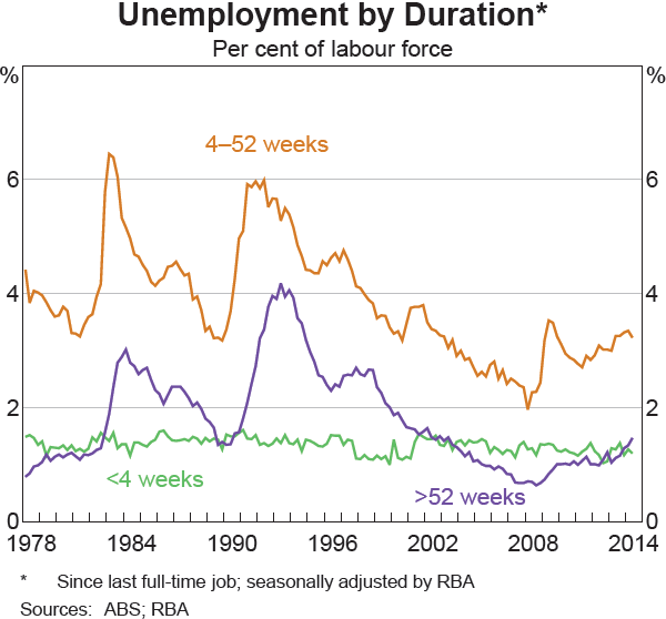
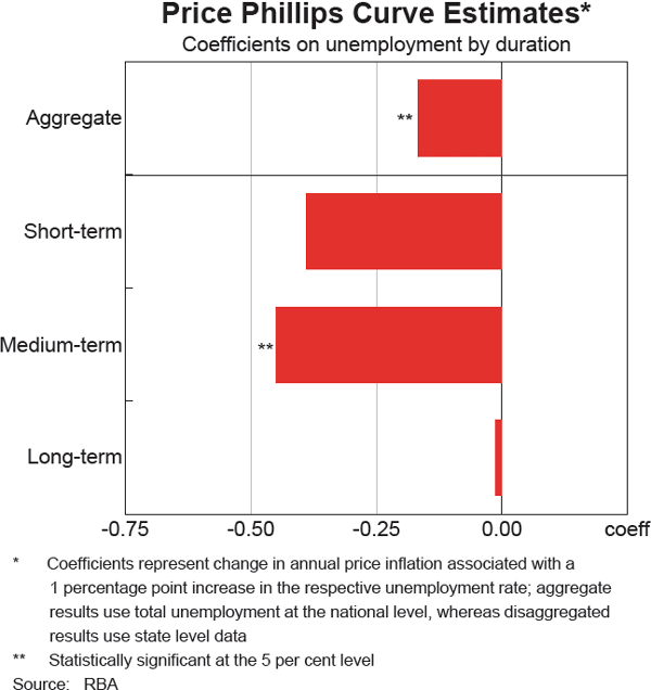
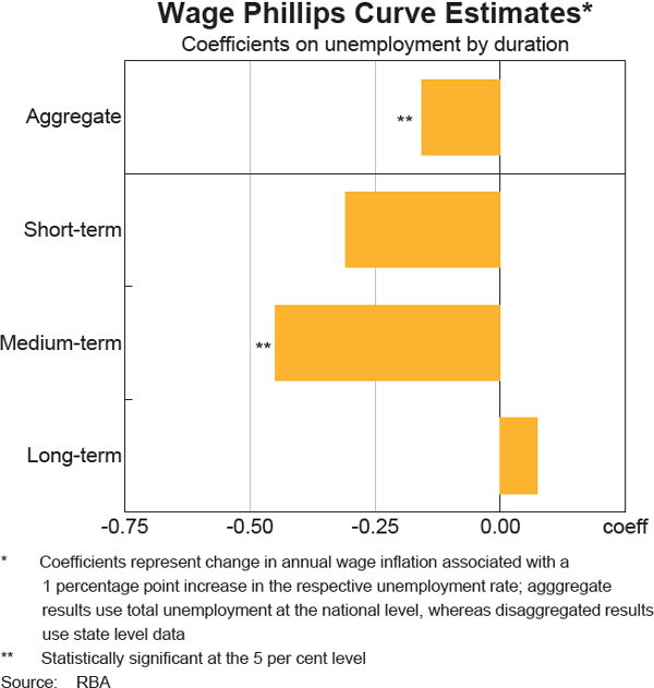
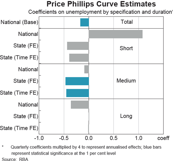
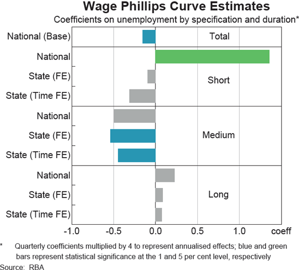
The statistical results appear to bear out these differences. Medium-term unemployment has a strong negative relationship with inflation, both in prices and wages (Graph 5 and Graph 6). On average, a 1 percentage point increase in the medium-term unemployment rate is associated with a reduction in both wage and price inflation of a little under ½ a percentage point (in annualised terms). In contrast, the long-term unemployment rate does not have a statistically significant relationship with inflation, which is consistent with these individuals having less of a bearing on wage setting. The short-term unemployment rate has a negative relationship with wage and price inflation, but it is not statistically significant and is less robust.[9]
Reason for unemployment
A drawback of the duration data is that they only provide information about the length of a continuous spell of unemployment. Short-term unemployment, for example, will include people that have recently resigned from their job in order to look for another job for frictional reasons. However, it will also capture people that have been recently retrenched, started looking for work for the first time, or have been out of work for a long time but were previously discouraged from searching. These groups are all likely to reflect spare capacity to differing degrees. Accordingly, it is useful to look at the reasons for unemployment, which include the following four categories:
- Those who worked in the past two years and left their last job involuntarily (e.g. were retrenched). This component may be a reasonable proxy for spare capacity in the labour market; as described above, when firms are looking to adjust to a fall in demand they will retrench more workers than usual, and vice versa. As would be expected, this component has been highly cyclical over time and is usually the largest group of those unemployed (Graph 7).
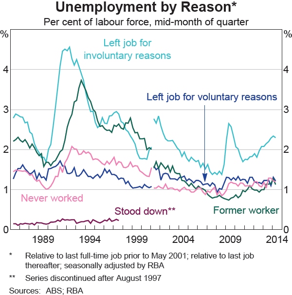
- Those who worked in the past two years and left their last job voluntarily (e.g. resigned). Voluntary job leavers are more likely to be frictionally unemployed, leaving a job to seek a better opportunity. This type of unemployment has been relatively stable over time, at 1–1½ per cent of the labour force.
- Former workers, who have worked previously, but not in the past two years. These individuals are more likely to be structurally unemployed and detached from the labour market for the reasons described above for long-term unemployment. Unlike long-term unemployment, this component will capture those individuals that have stopped searching for a job for a period while they have been out of work.
- Those that have never worked and are looking for a job for the first time.
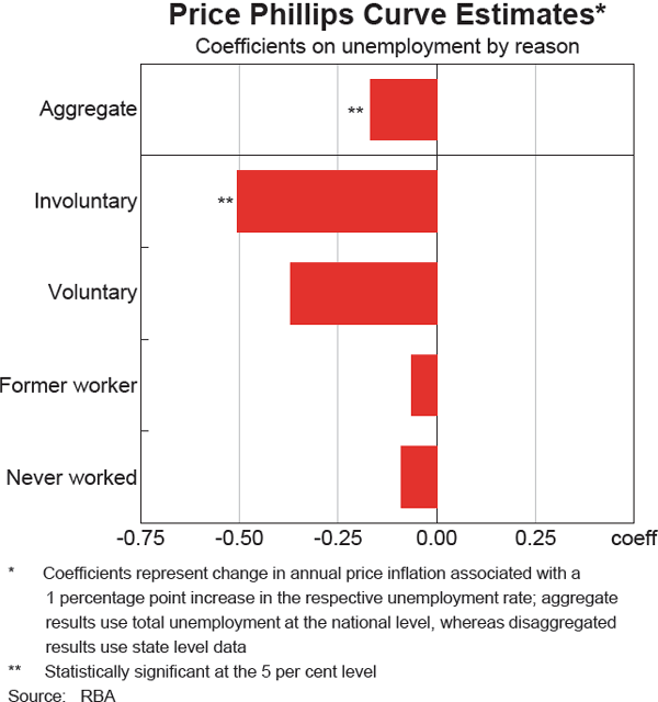
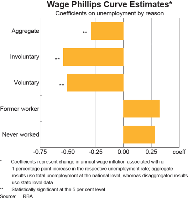
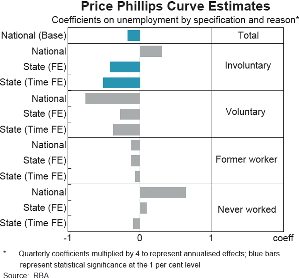
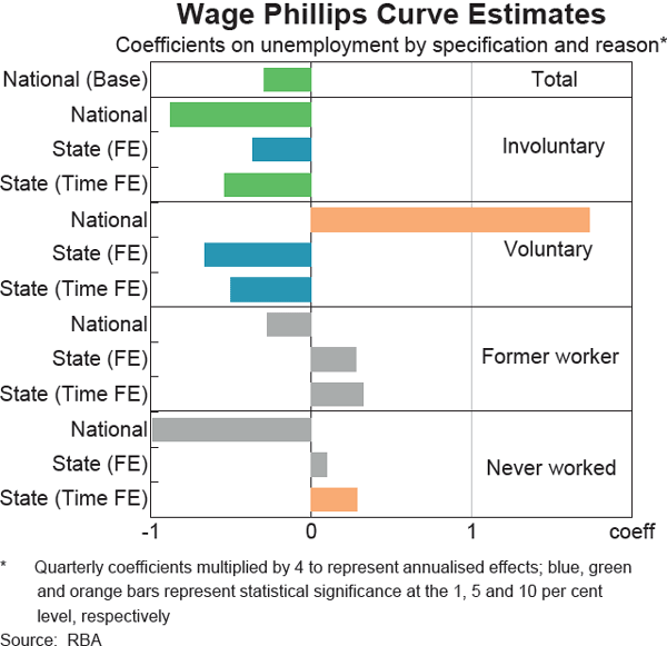
As expected, unemployment for involuntary job leavers has a strong negative relationship with price and wage inflation, suggesting that it is more likely to reflect the extent of spare capacity (Graph 8 and Graph 9). Unemployment for voluntary job leavers also has a negative relationship with inflation, although this is not as robust or statistically significant across models. In contrast, unemployment for former workers and for those that have never worked before seems to have a relatively weak relationship with inflation, consistent with these people being less influential for wage outcomes.
Factors affecting unemployment
Finally, we can break down unemployment by the obstacles that jobseekers perceive to be preventing them from finding a job. These can be grouped into three categories:
- A lack of labour demand, resulting in a general scarcity of vacancies or too many applicants for available vacancies. This category might be expected to be a reasonable measure of spare capacity in the labour market.
- A perceived mismatch between the individual and the available vacancies. In turn, this mismatch could be due to characteristics of the jobseeker, such as their experience, or due to the various requirements of the job. These individuals may face unemployment for more structural reasons, although they may be frictionally unemployed owing to the usual difficulties of searching for work.
- No reported obstacles, which might be indicative of frictional unemployment.
Unemployment influenced by a lack of labour demand has been particularly cyclical, rising sharply with the early 1990s recession, declining to very low levels by the mid 2000s, before rising again at the outset of the global financial crisis (Graph 10).
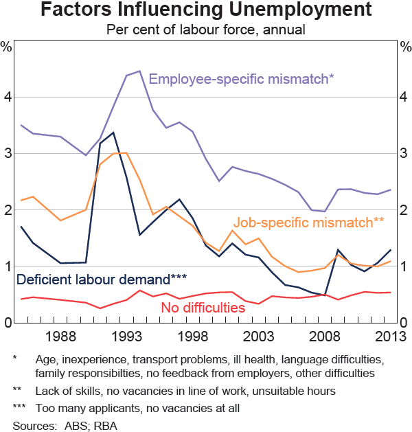
Unemployment influenced by mismatches between employees and jobs increased somewhat after the early 1990s recession, perhaps due to hysteresis, but has declined steadily since and has been stable since the mid 2000s. Finally, jobseekers reporting ‘no difficulties at all’ have been remarkably stable over time. While these data are conceptually relevant to the causes of unemployment, reliable Phillips curve estimates are difficult to produce because the data are only annual.
Interpreting Unemployment over the Past 25 Years
This article has outlined two approaches to assessing the extent of spare capacity in the labour market based on the unemployment rate. One is derived from statistical estimates of the NAIRU, the other comes from analysing the composition of unemployment. These approaches can be used to examine historical developments in unemployment.
At the outset it is important to reiterate that it is difficult to draw any strong conclusions. On the one hand, empirical estimates of the NAIRU are imprecise – the estimates have wide confidence bands, and the results can vary substantially depending on what measure of inflation is used and how the model is set up. On the other hand, the composition of unemployment is subject to uncertainty, as the observable components of unemployment do not provide conceptually ‘clean’ measures of spare capacity. In particular, the boundaries between the different causes of unemployment are inherently blurred. Finally, particular caution should be exercised when thinking about recent developments given the sensitivity of some of these indicators to new information and the propensity of model estimates to be revised.
With this in mind, the various indicators of cyclical unemployment suggest several distinct cycles in labour market spare capacity over the past 25 years (Graph 11).
- The 1990s saw significant spare capacity in the labour market. The unemployment rate was above several estimates of the NAIRU, particularly early in the decade. At the same time, the components of unemployment that are more indicative of spare capacity were also relatively high. Both of these approaches provide evidence of spare capacity, which is consistent with the relatively moderate domestic inflationary pressures and slow growth in labour costs seen over much of the decade. However, given the earlier experience of relatively high inflation, inflation expectations declined only gradually (Stevens 2003).
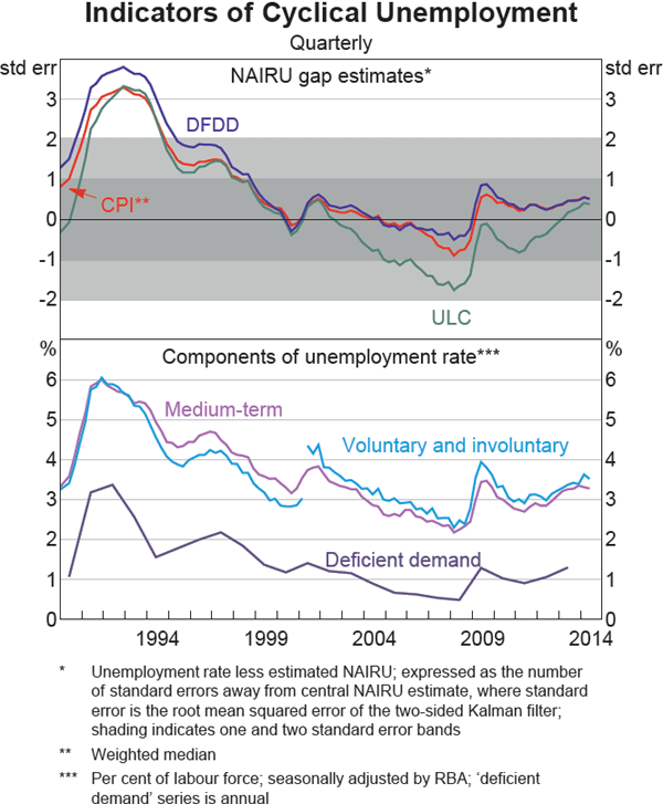
- The extent of spare capacity gradually moderated over the 1990s, and for much of the 2000s there was general evidence of labour market tightness. The unemployment rate fell below most estimates of the NAIRU, although not by enough to be considered statistically significant. At the same time, other indicators of cyclical unemployment were at low levels relative to their history. Consistent with this evidence of a tight labour market, the period ended with a rise in domestic wage and inflationary pressures (Lowe 2011).
- Since the global financial crisis, there appears to have been a degree of spare capacity in the labour market. However, this has been substantially less than was the case over much of the 1990s. The unemployment rate has recently been a little above several central estimates of the NAIRU (again these recent NAIRU estimates should be viewed with particular caution given their sensitivity to new information). At the same time, the more cyclical components of unemployment have also risen, accounting for most of the increase in the aggregate unemployment rate. This is consistent with evidence of subdued domestic inflationary pressures, including a slowing in wages growth and non-tradables inflation (Jacobs and Williams 2014; Kent 2014).
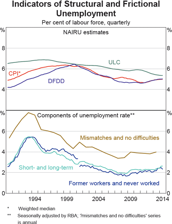
There is evidence that some changes in the unemployment rate have not been associated with a shift in spare capacity (Graph 12). Various estimates of the NAIRU increased over the course of the 1990s, and then declined over the 2000s. Similarly, components of the unemployment rate that are more structural also rose over the early 1990s, before declining gradually. More recently, estimates of the NAIRU and analysis of the composition of unemployment suggest that structural unemployment may have increased a little, but it remains low relative to history. There are various plausible reasons as to why structural and frictional unemployment might change over time, although again it is difficult to attribute changes to particular causes. Some possible contributing factors, which have been widely discussed in the past, include:
- Hysteresis. One important factor over time may have been hysteresis. Cyclically higher unemployment in the early 1990s might have had an enduring effect on the employability of jobseekers. Subsequently, an improvement in economic conditions over an extended period may also have worked to lower structural unemployment; a generation of individuals enjoyed good employment opportunities, meaning that relatively few endured a stint of damaging, longer-term unemployment.
- Economic reform. The ongoing benefits of economic reforms may have lowered structural unemployment over the past decade or so. However, the timing and magnitude of this effect are difficult to assess empirically (Borland 2011).
- Search technology. An improvement in search technology might have improved the efficiency of matching over time, lowering the unemployment rate. However, evidence for this effect is not clear, as the more ‘frictional’ components of the unemployment rate do not appear to have fallen over time.
- Changes in labour supply. The nature of spare capacity in the labour market may have changed over this period. There is evidence that ‘underemployment’ and ‘marginal attachment’ have risen relative to unemployment over time (Borland 2011). As a result, a given degree of overall spare capacity in the labour market might have become associated with a lower unemployment rate than previously.
- Structural change. Working in the other direction, the past decade has seen an increase in the pace of structural change in the economy, associated with the terms of trade boom (Connolly and Lewis 2010). This might have reduced the efficiency of matching between workers and vacancies, placing upward pressure on structural unemployment.
In summary, while it is difficult to be definitive, these indicators can be combined to enhance our understanding of movements in the unemployment rate.
Appendix A: NAIRU Estimation Framework
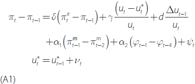
The methodology of Gruen, Pagan and Thompson (1999) is used to estimate the NAIRU for Australia. The following two-equation system is estimated:
where π represents the year-ended inflation rate, φ is quarterly inflation, π m is year-ended import price inflation, u is the unemployment rate, and u* is the NAIRU. Inflation expectations, π e, are taken as the break-even rate on indexed bond yields for a constant 10-year maturity. The NAIRU evolves as a random walk process. Gruen, Pagan and Thompson (1999) use underlying inflation, as measured by the CPI excluding interest and volatile items, and unit labour costs to estimate Phillips curves. In this article, the weighted median CPI measure is used to represent underlying inflation and an additional measure of price inflation, in the domestic final demand deflator, is included to complement these measures. The unit labour cost specification has a number of slight differences to the CPI specification, as set out in Gruen, Pagan and Thompson (1999).
The equations are estimated using maximum likelihood with a Kalman filter. The Kalman filter takes an initial value of the NAIRU, and in each successive period it estimates a NAIRU which enables the Phillips curve to fit the data as closely as possible. After stepping through the sample, from the first observation to the last, the ‘two-sided’ Kalman filter employed here then steps backwards, from the last observation to the first, to generate a smoothed NAIRU series informed by the full sample.
Appendix B: Phillips Curve Tests for Components of Unemployment
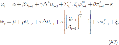
Phillips curves are widely used by central banks (after Phillips (1958); for a retrospective, see Fuhrer et al (2009)). For Australia, Phillips curves have typically been estimated using national level data with the aggregate unemployment rate (Gruen et al 1999; Norman and Richards 2010). For this article, the following price and wage Phillips curve specifications are estimated:
where φ is quarterly price inflation as measured by the headline CPI excluding volatile items, w is quarterly wage inflation as measured by the private sector wage price index, and u is the unemployment rate. Inflation expectations, πe, are taken as the break-even rate on indexed bond yields for a constant 10-year maturity. The price Phillips curve includes terms to account for the lagged effect of quarterly import price inflation (φm) constrained to follow a quadratic polynomial function. The wage Phillips curve includes a four-quarter geometric mean of the GDP deflator, g, to account for changes in the relative price of firms' output with respect to wages.[10]
Baseline specifications are estimated for aggregate unemployment at the national level. To test for different effects of the components of unemployment, the aggregate variable, u, is replaced by the decomposed unemployment rates (by duration or reason), with separate coefficients estimated for each component. The availability of data also necessitates slightly different sample periods for each regression: March quarter 1991–June quarter 2014 for the duration and reason decompositions with price inflation; December quarter 1997–June quarter 2014 for the duration decomposition with wage inflation; and December quarter 2001–June quarter 2014 for the reason decomposition with wage inflation.
As discussed above, some components of unemployment move closely with one another, resulting in a problem of multicollinearity. To address this problem, we follow the approach of Kiley (2014) for US data and make use of data at a more disaggregated level, for individual states. This approach includes state-level prices, wages and unemployment, but retains national-level inflation expectations, import prices and output prices. Two different state-level specifications are conducted. The first controls for any permanent differences in the level of inflation between states (i.e. state fixed effects (FE)). The second controls for time-varying factors that may affect wage or price inflation across all states and correlate with unemployment levels, such as changes to industrial relations laws (i.e. time fixed effects). The full results are shown in Graphs B1 to B4. Multicollinearity is evident in the national results, with coefficients often statistically insignificant individually but jointly significant, and with the opposite sign to that expected. All of the results are stronger at the state than the national level, with coefficients more stable and more significant. The state results are relatively similar for both approaches, so only one of these models (the time fixed effects model) is presented in the main body of the article.
Footnotes
The authors are from Economic Analysis Department. [*]
One indication of changes in matching efficiency is the Beveridge curve. For a discussion of developments in the Beveridge curve in Australia over time, see Borland (2011) and Edwards and Gustafsson (2013). [1]
To the extent that structural unemployment reflects hysteresis, a period of stronger demand might see some decline in structural employment. [2]
For a recent discussion, see Kent (2014). [3]
In turn, this will also place further downward pressure on price inflation, both because of more subdued growth in firms' labour costs, and because slower growth in household incomes and aggregate demand will weigh on firms' margins. Ultimately, low inflation may feed into expectations, further lowering inflation. [4]
Other changes can also shift the simple Phillips curve relationship, including changes in inflation expectations and import prices. In the statistical estimates of the Phillips curve set out in Appendix A, these influences are controlled for with additional regressors. [5]
For example, see Espinosa-Vega and Russell (1997), Ball and Mankiw (2002), Connolly (2008) and Farmer (2013). [6]
Previous work considering information contained in the composition of unemployment includes Connolly (2011). Unemployment data by duration and reason are published monthly and quarterly, respectively, in the Labour Force survey (ABS Cat No 6202.0), while factors contributing to unemployment are published annually in the survey of Job Search Experience (ABS Cat No 6222.0). [7]
These data are for duration since last full-time job. A shorter time series is available for duration since last full-time or part-time job. [8]
Some previous work for other countries finds duration of unemployment to be important for inflation (see, for example, Llaudes (2005)). In contrast, Kiley (2014) finds short- and long-term unemployment exert similar pressure on price inflation. [9]
The specification used here imposes a linear relationship between unemployment and inflation. However, if the relationship also depends on the level of unemployment, then it may be non-linear (Debelle and Vickery 1997). [10]
References
Ball L and NG Mankiw (2002), ‘The NAIRU in Theory and Practice’, Journal of Economic Perspectives, 16(4), pp 115– 136.
Blanchard O and P Diamond (1994), ‘Ranking, Unemployment Duration, and Wages’, Review of Economic Studies, 61(3), pp 417–434.
Borland J (2011), ‘The Australian Labour Market in the 2000s: The Quiet Decade’, in H Gerard and J Kearns (eds), The Australian Economy in the 2000s, Proceedings of a Conference, Reserve Bank of Australia, Sydney, pp 165–218.
Connolly E and C Lewis (2010), ‘Structural Change in the Australian Economy’, RBA Bulletin, September, pp 1–9.
Connolly G (2008), ‘Is the Trailing Inflationary Expectations Coefficient Less than One in Australia?’, Paper presented to the 37th Australian Conference of Economists, Gold Coast, 30 September–3 October.
Connolly G (2011), ‘The Observable Structural and Frictional Unemployment Rate (OSFUR) in Australia’, Paper presented to the 40th Australian Conference of Economists, Canberra, 11–13 July.
D'Arcy P, L Gustafsson, C Lewis and T Wiltshire (2012), ‘Labour Market Turnover and Mobility’, RBA Bulletin, December, pp 1–12.
Debelle G and J Vickery (1997), ‘Is the Phillips Curve a Curve? Some Evidence and Implications for Australia’, RBA Research Discussion Paper No 1997-06.
Edwards K and L Gustafsson (2013), ‘Indicators of Labour Demand’, RBA Bulletin, September, pp 1–11.
Espinosa-Vega M and S Russell (1997), ‘History and Theory of the NAIRU: A Critical Review’, Federal Reserve Bank of Atlanta Economic Review, Second Quarter, pp 4–25.
Farmer R (2013), ‘The Natural Rate Hypothesis: An Idea Past its Sell-by Date’, Bank of England Quarterly Bulletin, 53(3), Q3, pp 244–256.
Fuhrer J, Y Kodrzycki, J Sneddon Little and G Olivei (2009), ‘The Phillips Curve in Historical Context’, in Understanding Inflation and the Implications for Monetary Policy, A Phillips Curve Retrospective, MIT Press, Cambridge
Gillitzer C and J Simon (forthcoming), ‘Inflation Targeting: A Victim of its Own Success’, Paper presented to the Reserve Bank of New Zealand Conference, ‘Reflections on 25 Years of Inflation Targeting’, Wellington, 1–3 December.
Gruen D, A Pagan and C Thompson (1999), ‘The Phillips Curve in Australia’, RBA Research Discussion Paper No 1999-01.
Jacobs D and T Williams (2014), ‘Determinants of Non-tradables Inflation’, RBA Bulletin, September, pp 27–38.
Kent C (2014), ‘Cyclical and Structural Changes in the Labour Market’, Address on Labour Market Developments, hosted by The Wall Street Journal, Sydney, 16 June.
Kiley M (2014), ‘An Evaluation of the Inflationary Pressure Associated with Short- and Long-term Unemployment’, Federal Reserve Board Finance and Economics Discussion Series No 2014-28.
Ljungqvist L and T Sargent (1998), ‘The European Unemployment Dilemma’, Journal of Political Economy, 106(3), pp 514–550.
Llaudes R (2005), ‘The Phillips Curve and Long-term Unemployment’, European Central Bank Working Paper Series No 441.
Lowe P (2011), ‘Inflation: The Recent Past and the Future’, Keynote Address to BankSA ‘Trends’ Business Luncheon, Adelaide, 24 June.
Norman D and A Richards (2010), ‘Modelling Inflation in Australia’, RBA Research Discussion Paper No 2010-03.
Phillips AW (1958), ‘The Relationship between Unemployment and the Rate of Change of Money Wage Rates in the United Kingdom, 1861–1957’, Economica, 25(100), pp 283–299.
Pissarides C (1992), ‘Loss of Skill During Unemployment and the Persistence of Unemployment Shocks’, The Quarterly Journal of Economics, 107(4), pp 1371–1391.
Stevens G (2003), ‘Inflation Targeting: A Decade of Australian Experience’, RBA Bulletin, April, pp 17–29.
