RDP 2025-02: Boundedly Rational Expectations and the Optimality of Flexible Average Inflation Targeting Appendix D: Robustly Optimal Policy in the Unconstrained Case
April 2025
- Download the Paper 1.64MB
This appendix replicates the numerical results in Section 5 for the unconstrained case, where the central bank has perfect control of the output gap (i.e. perfect information and no ZLB).
D.1 Simple target criteria in the unconstrained case
Table D1 presents the optimal simple target criteria (defined in Table 2) under the baseline calibration. Optimal policy reduces the loss by 6.6 per cent compared to the loss under the IT rules. These gains can be almost entirely achieved by following a WAIT rule with a decay parameter of 0.52 (close to the share of rational agents, = 0.5). Placing additional weight on past output gaps or expected future inflation offers very small, if any, benefit. The importance of pre-emption is small when there is a reasonable share of rational forward-looking agents. The optimal pre-emptive respones to expected inflation can largely be achieved by a strong response to current and past inflation (especially because the cost-push shock is AR(1)). The price level targeting rule and especially the simple AIT rules perform poorly. Compared to the general case in Table 3, the optimal weight on lagged outcomes is smaller and IT performs better, which aligns with the analytical results in earlier sections.
| Rule | Loss (% relative to IT) | |||||
|---|---|---|---|---|---|---|
| 5-yr AIT | 96.5 | 31.3 | ||||
| 2-yr AIT | 48.8 | 13.0 | ||||
| 1-yr AIT | 7.7 | 21.5 | ||||
| PLT | 6.6 | 9.1 | 1 | |||
| IT | 0 | 11.6 | ||||
| IT + pre-emptive | –4.4 | 0.03 | 1.09 | 1.50 | ||
| WAIT | –6.6 | 8.4 | 0.52 | |||
| WAIT + WAXT | –6.6 | 8.4 | 0.53 | 0.01 | ||
| WAIT + pre-emptive | –6.6 | 8.2 | 0.52 | 0.33 | 1.02 | |
| WAIT + WAXT + pre-emptive | –6.6 | 8.2 | 0.52 | 0.00 | 0.33 | 1.02 |
| Optimal | –6.6 | |||||
| Notes: Welfare losses are normalised relative to the welfare under IT. The parameters for each rule are optimised to minimise welfare. | ||||||
D.2 Optimal policy under parameter uncertainty in the unconstrained case
Table D2 shows the average welfare and optimised parameter values for each target criterion when the policymaker is uncertain about expectations formation (i.e. across a set of different and g values). It also shows the average loss that would be achieved if the optimal criterion was implemented at each point of the grid, which represents the minimum loss achievable. As in the imperfect information case (Table 4), WAIT rules perform well, although the decay parameters are a bit lower at 0.56 to 0.67. Unlike the imperfect information case, there is little gain from making up for past output gaps via a WAXT component. This is consistent with the analytical optimal target criterion in result (17), in which no lagged output gap terms appear. The PLT rule performs poorly in the unconstrained case, and the 5-yr and 2-yr AIT rules always perform poorly.
Note that under the infinite-horizon Phillips curve, the optimal make-up weights in the unconstrained case are a bit larger (see Appendix C.2), so optimal policy in the unconstrained case is not as different from the constrained case.
| Rule | Average loss (% relative to IT) | |||||
|---|---|---|---|---|---|---|
| 5-yr AIT | 535.6 | 1.2 | ||||
| 2-yr AIT | 136.1 | 7.4 | ||||
| 1-yr AIT | 9.7 | 19.9 | ||||
| PLT | 4.2 | 10.9 | 1 | |||
| IT | 0 | 13.7 | ||||
| IT + pre-emptive | –0.4 | 3.0 | 14.9 | 0.42 | ||
| WAIT | –8.1 | 9.2 | 0.56 | |||
| WAIT + WAXT | –8.1 | 9.4 | 0.60 | 0.08 | ||
| WAIT + pre-emptive | –8.9 | 7.2 | 0.67 | 7.4 | 0.51 | |
| WAIT + WAXT + pre-emptive | –8.9 | 7.2 | 0.67 | 0.00 | 7.4 | 0.51 |
| Optimal | –13.7 | |||||
| Notes: The parameters reports are set to maximise the average loss across all points in the grid. Average welfare losses are normalised relative to the welfare under IT. | ||||||
To show what lies behind the average losses in the table, Figure D1 plots the loss under a selection of target criteria from Table D2 for different values of the expectation formation parameters and g. The parameters in the policy rules are held fixed at the robustly optimal values set to minimise average loss and not optimised for each and g shown in the figure. The dashed line shows the optimal target criteria optimised at each point to show how close the simple rules with the average coefficients can come to the fully optimal policy.
The IT rule performs well when is low, which is the expected result under adaptive learning. The PLT rule performs well when is high, close to the rational expectations benchmark, but unlike the constrained case, it performs quite poorly when is low. This is because nominal interest rate expectations are irrelevant when the central bank can perfectly control the output gap, so make-up commitments have zero effect when .
As in the constrained case, the WAIT rules perform consistently well across all parameter values. This is the case even though we have fixed the weight in the WAIT rules to the robustly optimal values in Table D2 so it is a fair comparison with the IT and PLT rules. Only in the optimal policy benchmark do we allow the policy rule parameters to change as we vary and g. The performance of the fixed-coefficient simple WAIT rules is remarkably close to the optimal benchmark, illustrating the robustness of this form of FAIT.
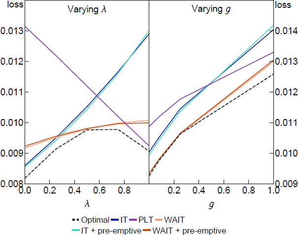
Notes: The parameters in the policy rules are fixed at the robustly optimal values presented in Table D2. For the other parameters (other than the one changing), we set = 0.5, g = 0.08, = 0.95, = 0.1, = 1, = 0.5, = 1 and = 0.1.