RDP 2024-06: Examining the Macroeconomic Costs of Occupational Entry Regulations 5 Examining the effects of OER
September 2024
- Download the Paper 1.59MB
As discussed above, occupational licences are intended to protect consumers, ensuring that goods and services meet a minimum quality by requiring providers to have a certain level of training. At the same time, occupational licences also impose economic costs. This stems from the greater difficulty for workers to switch and enter occupations with more stringent OER, which must be weighed against their potential benefits.
We provide the first empirical evidence for Australia on some of the potential costs of OER. We focus on two different aspects. First, whether more stringent OER reduce economic dynamism – that is the rate at which businesses enter and exit, or the rate at which the most productive businesses expand, which are important contributors to growth in productivity. Second, whether more stringent OER could be contributing to skills shortages that make it harder for those unemployed to secure employment.
5.1 Stringent OER make businesses less dynamic
We focus on economic dynamism for three reasons. First, there is a strong basis for a relationship. OER reflect a cost for workers to enter an occupation, making entry of new businesses more costly. Such barriers should also weaken the relationship between firm growth and productivity (Decker et al. 2020). Second, Bambalaite et al. (2020) find evidence of a relationship between OER and measures of dynamism. And third, measures of economic dynamism have been declining in recent years, with negative implications for productivity and living standards (e.g. Andrews and Hansell 2021). As such, understanding OER's relationship with these measures is of particular interest, as it may help us to better understand the slowdown in productivity observed over recent decades.
For this analysis we follow Bambalaite et al. (2020) and focus on a subset of the OECD occupations that can be easily mapped to commonly used industry classifications (ANZSIC – Australian and New Zealand Standard Industrial Classification). This mapping is shown below in Table 6.[5] Our sample includes observations for New South Wales, Victoria, and Queensland.
| Occupation | ANZSIC industry code |
|---|---|
| Baker | 1172, 1174 |
| Butcher | 4121 |
| Electrician | 3232 |
| Hairdresser | 9511 |
| Painter | 3244 |
| Plumber | 3231 |
| Taxi driver | 4623 |
| Accountant | 6932 |
| Architect | 6921 |
| Civil engineer | 3101, 3109, 6923 |
| Lawyer | 6931 |
| Real estate agent | 6711, 6712, 6720 |
|
Source: NSW Treasury and the Reserve Bank of Australia, data: ABS (2006). |
|
5.1.1 OER reduce business entries and exits
Occupational restrictions represent a barrier to entry for firms, creating costs for business owners in terms of their own training and potentially limiting the pool of qualified labour they can draw from. As such, we may expect entry rates to be lower where OER are more stringent. Exit rates may also be expected to be lower where OER are more stringent, given incumbents are protected from competition from entrants.
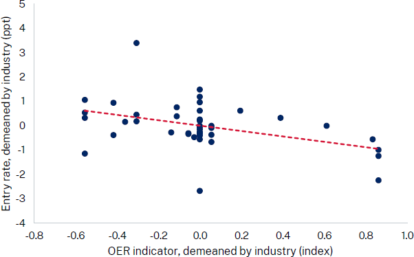
Figure 7 provides some initial evidence, plotting average entry rates over the period 2003 to 2019 for each industry-by-state pairing, alongside their OER.[6] In doing so we abstract from the average rates for each industry (remove industry means). This allows us to focus on differences across states with differing OER, rather than across industries where other factors may also influence entry and exit rates. We see that entry rates are lower the more stringent an occupation's OER.

Note: Each dot represents state-industry pairing. Entry rates are average from 2003 to 2019. Both entry rates and OER have mean level for industry (across states) removed. As such, chart focuses on differences in OER and entry rates across states, once accounting for average industry outcomes. Set of industry outlined in Table 6.
Source: NSW Treasury and the Reserve Bank of Australia.
To test this more formally we adopt a simple regression framework. The equation takes the form:
where Ratei,s is our measure of economic dynamism (i.e., entry and exit rates) in industry i, state s on average over 2003 to 2019, OER is the relevant OER measure, and captures industry fixed effects.[7] The coefficient of interest is , which captures whether entry and exit rates are higher or lower when OER are more stringent.
Table 7 shows the results. Our preferred model just focuses on how entry and exit rates and OER within each industry differ across states. So it just captures whether, for example, entry rates for hairdressers tend to be lower in New South Wales, which has more stringent OER for hairdressers, than Victoria and Queensland. But it will ignore the fact that OER scores and entry rates might tend to be low for hairdressers across all states on average. We find that a one-unit increase in the OER is associated with a 1.1 percentage point decrease in the entry rate and a 0.5 percentage point decrease in the exit rate. This is consistent whether we focus on all firms, or just employing ones.
| All firms | Employing firms | |
|---|---|---|
| Entry rate | −1.11*** | −1.13*** |
| (Standard error) | (0.38) | (0.40) |
| Industry controls | ||
| Observations | 42 | 42 |
| R-squared | 0.798 | 0.862 |
| Exit rate | −0.50* | −0.54* |
| (Standard error) | (0.25) | (0.29) |
| Industry controls | ||
| Observations | 42 | 42 |
| R-squared | 0.898 | 0.903 |
|
Note: (a) Standard errors in parentheses, ***P < 0.01; **P < 0.05; *P < 0.1. Standard errors are robust to heteroskedasticity. Coefficients represent percentage point increase in entry/exit rates for one unit rise in OER index. Source: NSW Treasury and the Reserve Bank of Australia. |
||
To put the numbers in context, the OER index for hairdressers in New South Wales is 1.25 units higher than Victoria and Queensland. This is estimated to have reduced the entry rate of hairdressers in New South Wales by around 1.4 percentage points and exit rates by 0.6 percentage point. This is equivalent to 168 fewer entrants and 76 fewer exits in 2023.
To estimate the potential costs of OER, we assess how much higher entry and exit rates would be if each industry had their OER lowered to the lowest rate observed in Bambalaite et al. (2020). This assessment, based on the estimated coefficients above, provides a plausible benchmark on how low OER can be while still providing consumer and worker protections. An alternative benchmark could consider the increase in entry and exit rates if OER were reduced to zero; however, this was not pursued as the benchmark is likely to be unrealistic in practice.
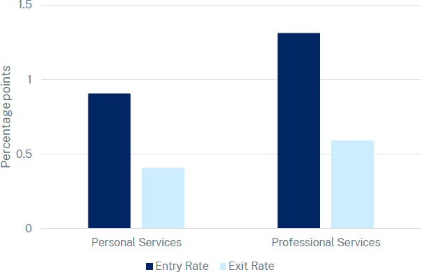
Figure 8 shows the outcomes. On average across the industries covered by our analysis, annual entry rates would be around one percentage point higher if OER rates were lowered to OECD lows. To put this in context, entry rates for employing businesses fell by around five percentage points from the mid-2000s to mid-2010s. So lowering OER could offset around one-fifth of the decline in economic dynamism observed over the past two decades, at least in those industries considered.
Similarly, exit rates would be around 0.5 percentage point higher. This is obviously a very simple, back-of-the-envelope partial equilibrium approach to quantifying the effect and should be interpreted in that context. But the results do suggest that reducing OER could have a notable effect on the entry and exit of businesses, at least in those industries considered.

Note: OECD lowest is average of five lowest scores across sample in OECD paper. Unweighted average across states and occupations.
Source: NSW Treasury and the Reserve Bank of Australia, von Rueden and Bambalaite (2020).
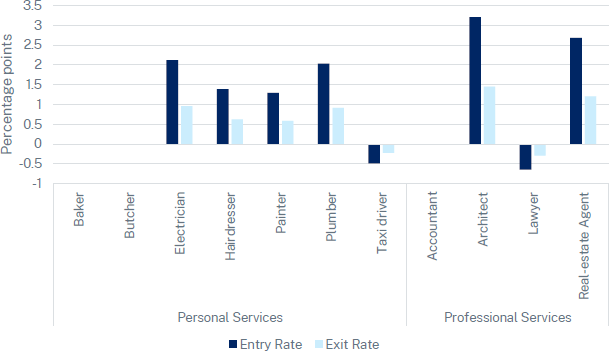
We can do a similar back-of-the-envelope exercise for individual industries, using the coefficient from the aggregate model and applying them to each sector (which may be a strong assumption). Aligning OER in New South Wales to those of the least stringent OECD countries would have the largest effects on entry and exit in the architecture and real estate industries (Figure 9). The entry rates for these occupations would be expected to increase 3.2 percentage points and 2.7 percentage points respectively. Across personal services, measures to relax OER would see greater business entry and exit among electricians, hairdressers, painters, and plumbers. This is noteworthy as New South Wales faces labour shortages in each of these occupations (National Skills Commission 2022). New South Wales has relatively more lenient occupational entry requirements for taxi drivers and lawyers, so there are no benefits to aligning these regulations to countries in the OECD.
This exercise is not arguing that OER should be loosened in these industries, as any assessment would need to weigh up these costs against the potential benefits, which is beyond the scope of this paper. It is simply trying to provide estimates and frameworks that can be helpful in any such assessments, and more generally to understand the effects of OER on the macroeconomy.

Note: OECD lowest is average of five lowest scores across sample in OECD paper. Unweighted average across states and occupations.
Source: NSW Treasury and the Reserve Bank of Australia.
5.1.2 OER make it harder for the most productive businesses to expand
OER could also affect the allocation of resources, creating frictions that hinder the rate at which highly productivity firms tend to grow. This is an important channel of productivity growth that can reduce the living standards of citizens. To examine the effects of OER and the flow of resources to more productive firms, we follow Bambalaite et al. (2020) and adopt the regression framework put forward by Decker et al. (2020).
This framework is motivated by standard models of firm dynamics which predict that, conditional on initial size, more productive firms should grow more quickly than less productive firms. But frictions that make it more costly for labour to flow between firms, or that weaken competition and therefore weaken the impetus for high-productivity firms to grow and make this gap in growth between high- and low-productivity firms smaller. This can lead to lower aggregate productivity growth as, all else equal, high-productivity firms will tend to be smaller and low-productivity firms larger.
The regression takes the form:
where is the employment growth of firm f in industry i, in state s, at time t, and Productivityf,s,c,t–1 is their labour productivity in the previous period. Xf,c,s,t contains a number of firm-level controls, including their size, and sales growth. are state and industry time fixed effects to capture the effects of the economic cycle on employment outcomes. As we include these industry controls, we are accounting for average growth and productivity in the industry, and so effectively are only comparing outcomes across high- and low-productivity firms within each industry, rather than capturing reallocation between more and less productive industries.
The coefficient of interest is , which captures whether the relationship between firm growth and productivity is stronger (>0) or weaker (<0) where OER are higher. In order to focus on the effects of the OER itself, we include an interaction between productivity and state unemployment. This allows us to abstract from the fact that the relationship between growth and productivity could vary depending on the strength of the local economy.[8]
In our preferred specification, similar to our entry and exit regressions above, we also control for the average strength of the relationship in each industry by interacting a dummy variable for each industry with the productivity term. This helps us to abstract from the possibility that some industries may, for some unrelated reasons, tend to have high OER and low rates of reallocation (e.g. due to high job-specfic human capital). Instead, we focus on how the rate of reallocation differs within industries across states, based on the differing OER level across states.
Table 8 shows the results. Focusing on our preferred specification in column 1, we see that more productive firms grow more quickly, but that this relationship is weaker where the OER is higher. To put numbers to this, take the case of a high- and low-productivity firm in an industry, where we define high and low productivity as one standard deviation above and below the industry mean (equating to around one log point either side of the mean). If we focused on an industry with an OER score of zero, the more productive firm would be expected to grow 10 percentage points faster – every year – than the low productivity firm. However, were the OER score to increase by one unit, this gap in growth falls to around nine percentage points.[9]
| Industry-by-productivity control | Industry-by-productivity control, since 2012 | |
|---|---|---|
| (1) | (2) | |
| Productivity | 4.71*** | 3.76*** |
| (Standard error) | (1.12) | (1.03) |
| Productivity*OER | −0.37** | −0.51** |
| (Standard error) | (0.15) | (0.22) |
| Controls | ||
| Productivity*lndustry | Y | Y |
| Observations | 708,591 | 406,903 |
| R-squared | 0.061 | 0.058 |
|
Note: (a) Standard errors in parentheses, ***P < 0.01; **P < 0.05; *P < 0.1. Standard errors clustered at the industry*state level. All regressions control for lagged firm sales growth and size, industry*state*year fixed effects, and productivity*state unemployment. Coefficients represent percentage point increase in employment growth for a one unit increase in log productivity. Source: NSW Treasury and the Reserve Bank of Australia. |
||
As with the entry and exit analysis, we can again ask: if OER were lowered to align with the lowest levels in the OECD, how much more quickly would labour flow from low- to high-productivity firms? Based on the regressions above, the predicted gap in growth between a high- and low-productivity firm given the observed OER was 7.5 percentage points. After lowering the OER that gap would increase to around 8.5 percentage points, a moderate increase for those industries analysed.
To put these in context, Andrews and Hansell (2021) find that, on average across the entire non-resource, non-financial private sector, the employment growth gap between high- and low-productivity businesses fell from around nine percentage points in the mid-2000s, to around seven percentage points in the mid-2010s. Moreover, they find that this had a substantial effect on productivity growth, lowering it by around 0.25 percentage point. So taking this admittedly very simple approach to quantificiation, it would suggest that we could offset around half of this decline in productivity and dynamism by lowering OER to OECD lows, at least for those industries considered here.
5.2 Stringent OER may be contributing to skill shortages
OER can dissuade workers from entering an occupation by creating a barrier to entry. This has the potential to lead to a mismatch between the demand for certain occupations and skills and their supply, both in the shorter term as demand for certain skills ebbs and flows over an economic cycle, and potentially over the longer term as the economy undergoes structural change. Such skills shortages and mismatches have the potential to raise the structural level of unemployment and impinge on economic growth more generally. The NSW Productivity Commission and NSW Innovation and Productivity Council (2022) also found that overly stringent OER can lower the quality of services by reducing competition in the labour market or perversely incentivising consumers to use unlicensed services.
The relationship between OER and skills shortages is examined using occupation-level metrics provided by the National Skills Commission's Skill Priority List (2022). This approach is less rigorous than the firm-level analysis above, as we cannot rule out the possibility that high OER and high rates of skill shortages are both driven by some third factor, such as the nature of the training required for certain occupations and how it is provided. For example, the need to learn a lot of content and skills. However, this approach still provides suggestive evidence of the effect of OER stringency on skill shortages.
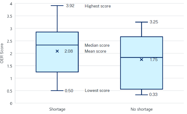
For this analysis we focus first on those sectors that are regulated by OER (i.e. have an OER indicator above zero). We focus on this subset to abstract from the variation in outcomes for unregulated sectors, which will be entirely driven by other factors. Overall, OER tend to be more stringent for occupations facing skill shortages than those not facing shortages (Figure 10). This suggests that OER may exacerbate skill shortages and could be contributing to higher levels of structural unemployment.
Considering occupations with OER, they are substantially experiencing skill shortages, compared to those without OER. For example, among the top 100 most common NSW occupations, only 30 per cent of the unregulated occupations were found to be facing skill shortages, compared to 75 per cent of the regulated occupations. Taken together these results provide some tentative evidence that more stringent OER may contribute to skill shortages.

Note: The chart examines OER stringency for 40 of the top 100 most commonly regulated occupations in New South Wales (i.e. all occupations with an OER stringency score > 0). The chart segregates OER stringency scores by occupations experiencing skill shortages and no skill shortages based on data from the National Skills Commission.
Sources: NSW Treasury and the Reserve Bank of Australia.
Footnotes
Relative to Bambalaite et al. (2020) we exclude driving instructors, as they are included in ANZSIC group 8219 ‘Community and Other Education’, which is very broad. [5]
For this analysis we exclude civil engineers as our sample is dominated by the mining boom, which will have substantively increased demand for and entry of such businesses in Queensland. [6]
Note that the evidence is weaker if we focus on the shorter sample since 2021. However, given volatility in entry and exit rates during the sample, our preferred approach is to focus over a longer period where these may average out. [7]
Unlike the entry regressions, we include civil engineering in these regressions as the inclusion of state by time, and state unemployment*productivity controls allow us to better account for the effect of local cycles. That said, results are very similar if civil engineering is excluded. [8]
More precisely, given the inclusion of the industry*productivity and unemployment*productivity variables, the numbers referred to are for a base industry, when unemployment is zero. Changing these parameters would scale up or down the level but would not change the effect of moving the OER. [9]