RDP 2024-03: Demand in the Repo Market: Indirect Perspectives from Open Market Operations from 2006 to 2020 3. Estimating the Demand Curve in Open Market Operations
May 2024
- Download the Paper 4.51MB
We derive an estimate of a downward sloping demand curve for liquidity obtained under repo in Reserve Bank open market operations. Since this involves cumulating successive bids at the auction, and our approximation of demand is imperfect, we also refer to this as a cumulative bid function (CBF). The CBF shares many similarities with demand curves and can be thought of as the sum over all participants' individual bid functions.[7] An individual participant's bid function captures the prices and quantities submitted at Reserve Bank auctions.
3.1 Methodology to construct the cumulative bid function
We begin by defining coordinates for the CBF, for the auction on day t, using individual bid-level data:
To illustrate the first part of this calculation, we use a hypothetical auction shown in Table 1. Each row lists a unique repo rate as a spread to overnight indexed swaps and the corresponding bid amount. Repo rates are ranked in descending order. In the third column, the cumulative value of the bids is calculated.
| Repo rates(a) (bps) |
Bid amount ($m) |
Cumulative bids ($m) |
|---|---|---|
| 25 | 200 | 200 |
| 24 | 250 | 450 |
| 23 | 100 | 550 |
| 22 | 600 | 1,150 |
|
Note: (a) In descending order as a spread to overnight indexed swaps. |
||
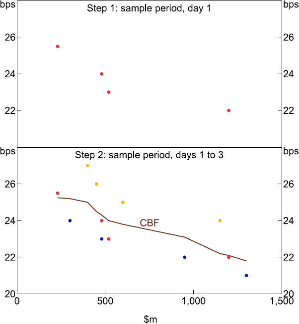
The CBF for this example involves plotting the four points (200, 25), (450, 24), (550, 23) and (1,150, 22). Each point on the CBF can be thought of as a marginal rate for each ranked approach and the corresponding total bid amount. For example, at a marginal rate equal to 25 basis points $200 million is bid, and similarly, at a marginal rate of 24 basis points $450 million is bid in total ($200 + $250).
In the next step to estimate a CBF over a specified sample period, we first plot all coordinate pairs for each day in the sample period, creating a scatter plot. Using this scatter plot, we estimate a curve by fitting a locally weighted regression (LOESS), with smoothing parameter = 0.75 and a quadratic specification.[8] This two-step process is illustrated in Figure 2 below.

Note: Each dot colour represents a different sample day.
3.2 Interpretation of the estimated curve
The shape of the curve reflects the cumulative quantity bid at different prices. It indicates the revealed willingness to pay at Reserve Bank auctions. While the revealed bid might not always be an exact reflection of the marginal valuation attached to repo funding, the overall interpretation as an estimate of demand is familiar (see also Appendix A).
The height of the curve approximates the willingness to pay for a given quantity of repo funding. A shift higher indicates an increased willingness to pay, which we associate with an increase in demand. In normal times there is probably little variation in demand for liquidity to meet underlying settlement and payment system obligations. It is more likely that demand for these purposes only rises noticeably during times of high uncertainty, as was the case in 2008–09 and early 2020. However, an increase in profitable investment opportunities in other markets that can be financed using repo might lead to a parallel upward shift. This could indicate a willingness to pay more for each dollar of repo funding to rechannel liquidity into another investment, either directly or through on-lending to clients.
The elasticity of the curve reflects the quantity response to a given price change. For a given decline in price, a negatively sloped and more elastic (flatter) curve is associated with a larger amount of repo funding contracted than when the curve is relatively inelastic (steeper). The curve might become more elastic when market participants become increasingly confident that funding obtained under repo can be rechannelled into secondary investments. That is, a small fall in the repo rate will be associated with a much larger willingness to borrow for reinvestment or on-lending when the curve is elastic.
Without pre-empting the statistical results in this paper, we note the importance of the basic theoretical point that an exogenous shock might simultaneously lead to both a shift in bids and changes in elasticity. We will revisit this point in the discussion of our findings.
The intersection between the demand and supply curves is where cumulative bids equal the allocation of cash supplied. It is an estimate of the cut-off rate, when all bids are filled from highest to lowest until the desired supply is exhausted.
Footnotes
See also Appendix A for the distinction between demand and the cumulative bid function. [7]
LOESS is a non-parametric method to fit a curve to a set of data points. The method assumes that points within a window are locally linear. The size of each window is equal to the parameter multiplied by the size of the dataset. The parameter also controls the smoothness of the curve. For further details, see Cleveland et al (1990). [8]