RDP 2022-05: The Real Effects of Debt Covenants: Evidence from Australia Appendix C: Trends before and after Treatments
October 2022
- Download the Paper 1,648KB
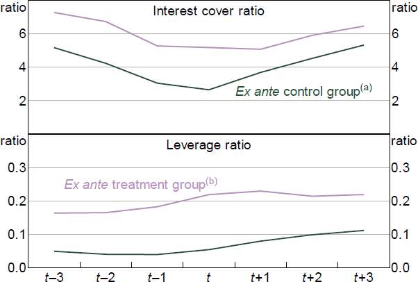
C.1 Test for parallel trends
To test for parallel trends before the covenants exposure treatment, I estimate the following regression on investment and staff expenses the years before the treatment:
The parameter of interest is the differential time trend coefficients, . The two groups follow parallel trends if the parameter is statistically significantly zero.
| Time trend coefficients | Difference |
||
|---|---|---|---|
| Control group | Treatment group | ||
| Investment | −0.0065863 (0.0071332) |
−0.0066515 (0.0071293) |
0.0000652 (0.0000284) |
| Staff expenses | −0.0114725 (0.0065714) |
−0.0115148 (0.0065660) |
0.0000423 (0.0000206) |
|
Note: Clustered standard errors at firm level are shown in parentheses. Sources: Author's calculations; Connect4; Morningstar |
|||

Notes:
(a) Defined as firms not exposed to covenants in both t – 2 and t – 1.
(b) Defined as firms not exposed to covenants in t – 2, exposed in t – 1 but no breaches in t – 1.
Sources: Author's calculations; Connect4; Morningstar

Sources: Author's calculations; Connect4; Morningstar