RDP 2022-03: Macrofinancial Stress Testing on Australian Banks 3. Credit Loss Modelling
September 2022
- Download the Paper 2,027KB
The main way in which macroeconomic downturns affect banks' balance sheets is through increased credit losses. In our stress testing model, credit losses are determined as the product of the estimated probability of default (PD) and the loss given default (LGD) for each of the bank's loan portfolios.[5] The framework we use is more complex for mortgages, business loans and commercial real estate (CRE) lending than for other portfolios because of the large contribution from these portfolios to overall credit risk. Since banks are required by accounting standards to provision for loan defaults before those defaults actually occur, the model also includes timing conventions to bring forward losses to the time when banks might reasonably recognise them.[6]
Sections 3.1 to 3.3 explain how the credit losses are estimated within the model for residential mortgages, business and commercial real estate lending, and other lending. Section 3.4 discusses when these losses are recognised as provisions.
3.1 Residential mortgages
There are two main options for modelling the PD on residential mortgages. One is to estimate a household-level or loan-level default model, using data from the Household, Income and Labour Dynamics in Australia (HILDA) Survey (as in Bilston, Johnson and Read (2015)) or the Securitisation Dataset.[7] The advantage of this approach is that it allows for a rich array of variables to influence defaults, including debt-to-income ratios, loan-to-valuation ratios (LVRs), borrower type and other household or loan characteristics. It also enables the scenario to incorporate changes in interest rates or fiscal policy, if desired. However, the drawback of this approach is that the loss rates such models produce tend to be much lower than rates observed either in previous global episodes of credit losses or in commercial banks' internal models of their own portfolios (e.g. Kearns, Major and Norman 2021). This may perhaps be because such models omit important features that matter in generating stress, or because the sample period over which they are estimated does not include enough variation in macroeconomic conditions to properly model tail risk. Regardless of the reason, the low loss rates mean we have not chosen to use this approach when modelling PDs on mortgages.
The alternative option, which we adopt, is to model PDs on residential mortgages as a calibrated function of just two variables: the unemployment rate and the LVR. The decision to use the assumed increase in the unemployment rate in the macroeconomic scenario as the key driver of defaults is consistent with a large literature on the drivers of housing loan arrears in both Australia (Bergmann 2020) and overseas (e.g. Ghosh 2015; Anastasiou, Louri and Tsionas 2016). The literature on household defaults also consistently find, however, that the sensitivity of PDs to the unemployment rate depends on the LVR of the mortgage; higher LVR loans are more likely to enter default than low LVR loans (Read, Stewart and La Cava 2014; Fuster and Willen 2017). This could to some extent reflect the incentive to strategically default when borrowers have little equity in their loan. However, given this empirical regularity is observed in jurisdictions that have both non-recourse and full-recourse lending, it is more likely to reflect that borrowers with larger amounts of equity are better able to self-cure than borrowers with little equity, or that borrowers with certain characteristics that make them more likely to default also tend to take on more leverage. Regardless, our approach of specifying PDs on mortgages to be a function of two variables enables us to link macroeconomic developments to defaults in a way that produces what we consider to be severe but plausible loss rates.
More specifically, the PD on mortgages that have an LVR within a specific bucket is measured as the rate at the onset of the scenario (derived from APRA data) plus an additional increment that is proportional to the change in the unemployment rate since that time.[8] The proportionality between the unemployment rate and this additional increment varies across the different LVR buckets, increasing as the LVR rises. We also constrain the PD to not fall below a base level that reflects the natural level of default that occurs even in a strong economy due to marital failure, illness, disability and other non-cyclical risk factors. Given all this, the PD for an LVR bucket k held by bank i at time t can be represented by:
where PDi0 is the initial (annualised) PD on that bank's (total) mortgage portfolio, is the increase in the unemployment rate from the beginning of the scenario to time t , is a coefficient that determines the sensitivity of the whole mortgage portfolio to rises in unemployment and is a vector of multipliers that capture the propensity of LVR bucket k to default relative to the whole mortgage book. Specifying the PD to be the sum of its initial value and the change in unemployment since the beginning of the scenario implies an assumption that the starting PD captures the effect of unemployment prevailing at the beginning of the scenario.[9]
The absence of historical experience with large losses on banks' mortgage portfolios makes calibrating difficult. Given this, we use a combination of approaches to calibrate this parameter. One approach is to adopt the estimates in Bergmann (2020), which uses the dispersion in Australian unemployment rates across regions to estimate the sensitivity of mortgage defaults to the unemployment rate. Bergmann's research implies a parameter of around 0.2. We consider this to be a lower bound, given Gyourko and Tracy's (2014) observation that using regional unemployment rates instead of individual unemployment rates can bias down the true effect of unemployment on losses. A second approach is to estimate a simple bivariate regression relationship between unemployment and non-performing loans across a wide range of countries, with a particular focus on those whose institutional and legal frameworks, LVR distribution, and borrower and bank characteristics are more similar to those in Australia. This results in coefficients of up to 1.0, depending on the specification and which countries are included. (Figure 2 displays the dataset considered for this regression; our coefficient estimates are largely derived from countries in the bottom half of the figure.) Our assessment is that this approach is likely to slightly overstate the sensitivity of Australian mortgages to rising unemployment. Given these considerations, we choose a parameter of 0.6, which is in between the two approaches but still conservative in our view.[10]
Our calibration of the vector is based more closely on the results of Bergmann (2020), which we judge to appropriately capture how the sensitivity of defaults to unemployment will vary with LVR during times of stress. We fit a quadratic function to the coefficients from Bergmann to produce a smoothly evolving vector of coefficients, with the choice of a quadratic function based on a visualisation of the data. This calibration results in loans with an LVR of around 100 per cent being about 1.5 times more likely to default than loans with an LVR of 60 per cent. This calibration from Bergmann is more muted than what could be imposed based on Read et al (2014); they estimate that loans with an LVR of 90–100 per cent are 3½ times more likely to default than loans with an LVR below 60 per cent. However, the latter estimate is based on a smaller sample of publicly traded residential mortgage-backed securities (RMBS), and selection bias in this sample (arising from incentives for RMBS issuers to only include high-quality loans) may plausibly bias this multiple higher compared with the sample of self-securitised RMBS used by Bergmann.
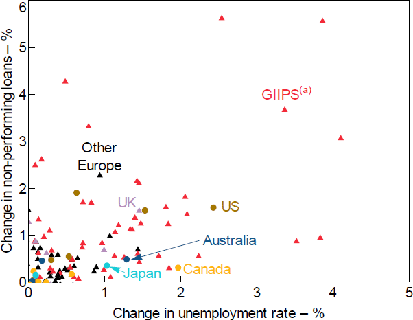
Note: (a) Includes Greece, Ireland, Italy, Portugal and Spain.
Sources: APRA; Authors' calculations; Bank of Canada; Board of Governors of the Federal Reserve System; S&P Global Market Intelligence
The LGD for banks' mortgages are driven by the assumed profile for housing prices, along with the starting LVR and an assumed value for banks' foreclosure costs. In particular, the model specifies that the LGD is equivalent to one minus one over the LVR prevailing after the shock to house prices (that is, the extent to which the borrower is in negative equity), plus a margin to cover foreclosure costs:[11]
We estimate dynamic LVRs (that is, current debt outstanding relative to the current value of the property) by extrapolating current LVRs (that is, current debt outstanding relative to the purchase price of the dwelling) reported in the Securitisation Dataset (see Fernandes and Jones (2018) for more details). This is done using housing price trends observed in the local area for each property since the loan was originated and our assumed profile for housing prices. Our estimate of foreclosure costs being 10 per cent is based on the international literature (Qi and Yang 2009) and assumptions used by Standard and Poor's and Fannie Mae, all of which show values in the range of 7 to 13 per cent. We take into account the benefits to banks of lender mortgage insurance (LMI) by applying a pre-specified recovery rate to mortgages that are covered by insurance and reducing LGDs.[12]
Loss rates are the product of these modelled PDs and LGDs, and are shown in Figure 3 for various assumed housing price profiles. The resulting loss schedule is broadly consistent with loss rates observed in various historical experiences (such as Australia in the global financial crisis and the United Kingdom in both the early 1990s and the global financial crisis) and with those estimated in various iterations of APRA's industry-wide stress tests. These profiles also highlight that large losses on mortgages only occur when there is both high rates of unemployment and large falls in house prices, consistent with previous research (Elul et al 2010; Bergmann 2020).
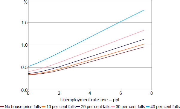
Note: Loss rate cumulated over 12 quarters.
3.2 Business loans and CRE loans
In the following paragraphs the estimation approach for business loan losses is outlined. The same approach (i.e. PDs and LGDs derived from this approach) is also used to estimate losses on CRE loans as it is likely that very similar dynamics will govern the loss rates for both loan categories.
Losses on business lending typically account for a disproportionately high share of total bank losses in recessions (Rodgers 2015). However, it is difficult to empirically calibrate a loss model from the experience of Australian banks' business losses, given declining business non-performing loans over the last decade, the absence of large losses in the past 30 years and the paucity of data from banks' experiences in the early 1990s recession (in addition to significant changes in lending practices since then). Perhaps because of this, models of defaults on business lending derived from firm-level databases (such as Kenney, La Cava and Rodgers (2016)) tend to be relatively insensitive to macroeconomic cycles, and do not produce much stress in recessions.
In light of this, our approach to modelling business defaults uses a multi-step process, with calibrations drawn from a wide range of domestic and international sources (as set out in Figure 4). The inputs to this model are the GDP growth shock derived in the scenario, the distribution of banks' exposures by internal credit ratings (as reported in Pillar III reports) and various coefficients that are drawn from Australian experience, the research literature and the Capital IQ database of global, firm-level credit ratings and experience. We use these inputs in a three-step process:
- Construct an implied distribution of interest coverage ratios (ICRs) for customers of each bank. (ICRs are defined as total interest payments divided by profits, and have historically been the best predictor of future default.)
- Update this distribution by mapping the assumed shock to GDP growth into an assumed distribution of firm-level shocks to earnings.[13]
- Apply a default rule to the updated distribution of firm ICRs by bank to determine the share of exposures that default.
These derived PDs are then combined with LGD assumptions derived from data on the security backing banks' lending to produce loss rates. The remainder of this section describes this process in more detail.
The first step in modelling PDs on business lending involves mapping banks' internal credit ratings to an implied distribution of ICRs. We begin by taking data on the internal credit ratings of banks' exposures from Pillar III reports. The internal credit rating grades used by banks (e.g. A-, BBB+), align with those reported in the Standard & Poor's Capital IQ database of global firms. The Capital IQ database also provides estimates of ICRs for each firm. There is a reasonably distinct (though overlapping) relationship between the distributions of ICR for each credit rating (after excluding utilities and financials), enabling us to imply a distribution of ICRs for the exposure of each bank within each credit rating.
The second step involves calculating the distribution of changes in earnings for banks' customers in the event of a recession. This is not the same as the assumed change in GDP in the scenario. One reason for that is the recognition that profits are typically procyclical, and hence will typically fall by more than the decline in GDP. Another reason is that some firms are more procyclical than others. We feel this latter point is essential for modelling defaults on banks' business lending portfolios, since large falls in earnings at some firms cannot be offset by increased earnings at others.
Given these observations, we introduce two features that translate the shock to GDP growth into a firm-level distribution of changes in earnings. The first is to map the GDP growth shock into an aggregate shock to firm profits. This can simplistically be done by regressing the time series of profit growth on GDP growth, using ordinary least squares. Such an approach implies that profits are about 50 per cent more cyclical than GDP, largely because a sizeable share of firms' costs (including wages) are fixed,[14] and this ratio is used to translate GDP growth shocks into aggregate profits growth shocks. The second feature is to create a distribution of shocks to firms' earnings, with its mean equivalent to the change in aggregate profits growth calculated so far. We calibrate the variance and skewness of this distribution from the international literature on how firm-level profits evolve during recessions. More specifically, we use the estimates from Bloom et al (2018).[15]
The first step allows us to calculate a starting distribution of ICRs for each bank's exposures by credit rating, while the second step updates that distribution to reflect the shock to profitability imparted by the assumed GDP profile. However, we require a third step to complete the default model: a rule that translates ICRs into PDs. In particular, we make the assumption that ICRs are determinative of default, which allows us to set an ICR threshold below which firms default on their loans. The assumption that ICRs are determinative of default is admittedly strict, but research has shown that ICRs are a strong predictor of default (Kenney et al 2016) and are the metric most commonly used by banks when assessing serviceability. The specific ICR threshold below which a firm is assumed to default is set at just under 2 times, based on Reserve Bank of Australia (RBA) internal research confirming an ICR of 2 to be the most informative in identifying failed companies.
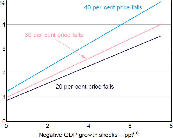
The representative profile of PDs for various GDP growth shocks that is derived from this approach is shown in Figure 5. This profile varies slightly across the size distribution of banks' loan portfolios, with smaller firms consistently having higher PDs than large corporates, based on the starting distribution of credit ratings reported by banks. However, all portfolios experience heightened defaults in response to recessions of the magnitudes experienced historically in Australia. For a 2 percentage point fall in year-ended GDP growth, the calculated PD increases by around 1 percentage point.[16] For a 7 percentage point fall in GDP growth the calculated PD increases by around 3 percentage points.[17] The profiles shown in Figure 5 sit a bit lower but are broadly consistent with both the rules-of-thumb in Hardy and Schmeider (2013) and from APRA's internal estimates of PD increases.
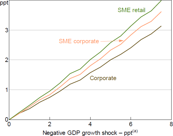
Note: (a) Year-ended GDP growth.
Another potentially important aspect that may influence business loan default rates is the industry composition of a bank's business lending. The model is flexible enough to incorporate different assumptions of default rates by industry for each size category of lending, modelling a downturn in the economy that is triggered by an industry-specific shock. For each size–industry category, the model multiplies the baseline default rate by a size–industry specific multiplier (by default this is set to one) that increases default rates in those specific industries relative to the baseline model. These increased default rates will then feed into overall default rates on the overall business portfolio, depending on the composition of an individual bank's business loan portfolio.
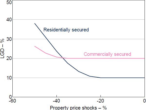
A separate LGD model is used to translate these PDs into loss rates. These LGD estimates are driven by two factors: an implied distribution of pre-shock LVRs based on data reported by banks; and estimates of the decline in property prices (both residential and non-residential) arising from the assumed macroeconomic scenario. There are no data we know that fully capture the distribution of pre-shock LVRs on banks' business loan portfolios. However, it is possible to infer a distribution using data reported to APRA and some assumptions. In particular, the data reported to APRA specify the share of banks' business lending that is fully secured, partially secured or unsecured, and these data are split by firm size category. We then assume that LVRs for fully secured loans to corporates are distributed uniformly between 35 and 65 per cent, while fully secured loans to SME retail firms are uniformly distributed between 60 and 80 per cent and the LVRs for SME corporates are assumed to be an average of the these two distributions. (These ranges are set based on information gleaned from RBA liaison with banks.[18]) These LVR distributions are then updated based on the scenario for property prices, assuming that the vast majority of secured loans are backed by some form of property. This assumption is also based on discussions with banks, who suggest that secured corporate loans are typically secured by commercial property, secured SME corporate loans are regularly secured by either residential or commercial property, and that secured SME retail loans are typically secured by residential property. In addition, we assume that banks incur foreclosure costs amounting to 20 per cent for business loans backed by commercial property collateral and 10 per cent for loans backed by residential collateral. Foreclosure costs for business loans backed by commercial property are assumed to be higher than those for residential mortgages because transaction costs for commercial property sales are significantly higher than those for residential property sales, and because commercial property is less homogenous than residential property and so more likely to require a discount to ensure a sale. The resulting mapping from property price shocks to LGDs on different types of loans is shown in Figure 6. For unsecured loans and partially secured loans, we assume a fixed 50 per cent LGD, which is broadly consistent with APRA's internal modelled results.
A final component of estimating business loss rates involves incorporating the potential usage of credit lines by corporates during macroeconomic stress events. The model typically uses data about on-balance sheet exposures of the banks to calculate losses, and so would often exclude credit lines. During the global financial crisis and the onset of the COVID-19 pandemic, however, firms used these lines significantly, illustrating the importance of accounting for these dynamics in stressed events (Minoiu and Kapan 2021). In recognition of this, the modelling approach incorporates the ability to specify both whether these lines are drawn down by firms in the starting period (i.e. are added to banks' exposures immediately) and what proportion of credit limits are actually drawn down by firms if they choose to. These exposures are then added to the stock of corporate credit (i.e. they attract the same default rates as corporate loans) and are assumed to have an LGD of 100 per cent. The latter assumption is adopted because it is likely that these lines of credit are unsecured, and likely to have lower recovery rates than outstanding unsecured loans.
The resulting schedule of loss rates for various falls in GDP and property prices is shown in Figure 7.
Notes:
Loss rate cumulated over 12 quarters.
(a) Year-ended GDP growth.
3.3 Other portfolios
For personal loans (including credit cards), unemployment is the main determinant of the ability of households to service debt obligations and, thus, probability of default (Banerjee and Canals-Cerdá 2012; Dinh, Mullineux and Muriu 2012). Indicative of this, there has historically been a tight relationship between the unemployment rate and credit card loss rates during stress events in many advanced countries (Bellotti and Crook 2013). Accordingly, we specify the PD on personal loans to be a function of just the unemployment rate. We assume that LGDs for these loans are fixed at bank-reported starting values, given they are unsecured. We benchmark losses to past APRA stress tests to arrive at calibrated coefficients for the PD model, and crosscheck our loss rates with estimates drawn from Bilston et al (2015). This results in a 1 percentage point higher unemployment rate leading to a 0.4 percentage point rise in the PD for personal loans.
For overseas exposures, we assume the loss rate is the average loss rate of the other asset classes that we have estimated. This implies that losses on foreign exposures are proportionate to losses on the equivalent domestic portfolio. Given the high degree of economic synchronicity between Australia and New Zealand (by far banks' largest offshore lending exposure), and the full-service nature of their New Zealand operations, this will rarely be problematic. However, it could reduce the accuracy of the results for a few banks with large Asian exposures, in a scenario where Asian economic conditions diverge from those in Australia. Similarly, the loss rate on domestic intragroup exposures is assumed to be the same as for equivalent loans to a third party; this is unlikely to be true, but the small scale of such loans means this simplifying assumption will rarely distort the model results. For other domestic loan types (such as loans to financial institutions), we make some simplifying assumptions in recognition these loans comprise less than 5 per cent of total loans. Specifically, we assume these loans PDs and LGDs stay constant at their starting rates over time.
3.4 The use of loan loss provisions
Accounting rules require banks to recognise loan losses before they actually materialise. This is done through the use of provisions. Banks must set aside some level of provision for all loans, but the rate of provisioning increases sharply as loans begin to show signs of elevated credit risk. This has the effect of bringing forward and concentrating losses in a smaller number of periods. As a result, it typically exacerbates the pace of decline that banks experience. Simulations suggest that forward-looking provisioning can plausibly lower the trough in bank capital ratios by up to 50 basis points, though this is subsequently unwound as the losses are realised without affecting profits over the long term.
The process by which loan loss provisions and bad debt charges are calculated in the model involves four steps:
- Loan write-offs for each portfolio during the current period are calculated using the loss models described above.
- The required loan loss provision balance is then calculated as the expected write-offs in each of the subsequent four quarters plus an additional balance to reflect the minimum level of provisions. The minimum level is included to ensure that banks retain some level of provision for lifetime losses (that is, beyond the next year), and is set at each bank's lowest historical level of provisions (relative to loans) for each asset class.[19] Expected write-offs are calculated using the loss models described above and an assumption that banks perfectly foresee the economic outcomes entailed in the model over the year ahead (so that their provisions match actual future outcomes).[20] The assumption of perfect foresight is clearly strong, but it is not clear that other potential assumptions are more realistic and it makes the modelling simpler. It is also not clear whether adding uncertainty would increase or decrease banks' provisions in the early stages of stress: uncertainty should arguably cause banks to hold excess provisions to account for the higher risk of large losses, but loss aversion could also cause banks to underestimate possible losses in the face of uncertainty.
- The increase in the loan loss provision balance is calculated as the difference between the balance calculated in step 2 and the prior period's provision balance. This can be negative when the macroeconomic outlook begins to improve.
- The bad debt charge is then calculated as net write-offs plus the increase in the loan loss provision balance. The balance for loans in each asset class is then updated by subtracting write-offs determined for this period from the balance of loans at the beginning of the period (plus any growth resulting from the reinvestment of profits).
The use of loan loss provisions is mandated in accounting standards, but tax rules do not allow banks to claim a deduction for losses arising from provisions on loans that are still performing. The difference between the accounting balance sheet and the taxable balance sheet is reconciled by creating a ‘deferred tax asset’, which is a record of the tax deduction that can be claimed in future if the loan does default. The deferred tax asset is not an asset that can be realised for value during insolvency and so is deducted from regulatory capital. In the model, this is accounted for by adding back changes in provisions when calculating taxes owed. This means that net profit after tax can be added to regulatory capital in the model without adjustment, since the difference between the taxable and accounting balance sheets is already accounted for when calculating profits.[21]
Footnotes
There is no real distinction in the model between PDs and default rates, so the two are used synonymously. [5]
For more information, please see AASB (2021, Chapter 5). [6]
Using the HILDA Survey allows the model to include a rich set of personal characteristics that can influence default rates and are not in the Securitisation Dataset, but at the cost of linking each loan to different banks. [7]
These LVR buckets are specified in 1 per cent increments from 1 per cent to 250 per cent. [8]
We choose to specify the PD as a function of the cumulative rise in unemployment, rather than the change over a few quarters, because financial buffers typically mean that it takes many quarters for people that lose their job to default. [9]
One of the reasons that we consider this parameter to be conservative is that it will result in the PD being persistently elevated by this amount when the unemployment rate is above its initial level. In contrast, the data in Figure 1 and Bergmann's results are both estimated from changes. We make this distinction to ensure that PDs don't fall to low levels as the unemployment rate begins to decline from an elevated level. [10]
This is a simplified version of the LGD calculation as it abstracts from lender mortgage insurance coverage that is accounted for in the model. See Appendix A for more details. [11]
The recovery rate is set at 66 per cent by default, but is a flexible parameter that allows various assumptions about the support that LMIs may provide to be modelled. [12]
To simplify the modelling, we assume interest rates on business loans do not change. This will likely mean losses are understated, but we think the effect is modest because earnings are typically much more volatile than interest rates. [13]
It is also possible to use quantile regression to estimate this sensitivity, given that earnings tend to weaken in the final stages of an expansion and so ordinary regression analysis may understate the sensitivity of profits to GDP shocks. Quantile regression at the 20th percentile implies that profits growth are 150 per cent more cyclical than GDP growth. [14]
A more complicated (and default-inducing) distribution can be derived from Bachmann and Bayer (2013), but for simplicity we do not use it in our analysis. They show that the variance and skewness of shocks to firm profits is dependent on the extent of the decline in GDP growth. [15]
Starting PDs are determined by data banks report to APRA and generally are in the range of 1 to 3 per cent depending on the bank. [16]
The mapping between GDP shocks and increases in PDs that our approach produces is close to linear, and so for modelling purposes we approximate it using a linear model. The lack of significant nonlinearity reflects that the increase in variance of profits as the GDP shock increases is still a linear function. Allowing the skewness of the profit distribution to change as the shock increases does induce more nonlinearity, but we choose to omit this feature for simplicity. Non-linearity is introduced in the translation of ICRs into default rates. [17]
This is simulated by drawing LVRs from a uniform distribution between 35 and 65 per cent and between 60 and 80 per cent, depending on the type of property. [18]
This is a simplification for modelling purposes. Higher provisions might be expected in a scenario in which credit risk is elevated, since banks are unlikely to assume this risk fully unwinds after a year. [19]
It's not straightforward to precisely model perfect foresight with nonlinearities, but we can approximate it. [20]
There will be a difference between profits calculated by this method and profits calculated for accounting purposes, with the difference being the size of the ‘deferred tax asset’ created. [21]