How Does Unemployment Affect Household Spending? | RDP 2021-08: Job Loss, Subjective Expectations and Household Spending

RDP 2021-08: Job Loss, Subjective Expectations and Household Spending 4. How Does Unemployment Affect Household Spending?

Gabrielle Penrose and Gianni La Cava

August 2021

Download the Paper 2,109KB

The next part of the paper explores the effects of unemployment, and expectations of job loss, on household spending. Understanding the relationship between household-level consumption, expectations and unemployment can shed light on how households make economic decisions, and test various theories of household consumption. While we have previously considered job loss, we now consider unemployment. This is primarily because the HILDA Survey asks about typical or current expenditure, meaning we are unable to observe consumption losses from unemployment spells that occur because of job losses between survey waves. To get around this, we focus only on workers who are unemployed as at the time of the survey. Despite this, we acknowledge that in some circumstances a job loss event may not be followed by unemployment (if the worker leaves the labour force, or finds new employment immediately), and in others unemployment may not be the result of job loss (if an unemployed respondent voluntarily left their previous job, for example).

In addition, the consumption response to unemployment may help us quantify the welfare effects of unemployment on households. Unlike current income, consumption relates directly to household welfare. This is because temporary fluctuations in income may be smoothed over the life cycle, while consumption is typically less volatile. To the extent that we want to capture the effect of unemployment on economic wellbeing, consumption is a better indicator.^[6]

4.1 Theoretical framework

To frame the analysis that follows it is useful to outline how household consumption responds to changes in income under the assumptions of a standard workhorse model, such as the PIH (Stephens 2004; Been et al 2020). In this set-up, households are assumed to be infinitely lived, face constant interest rates, have quadratic utility functions and supply labour perfectly elastically. The only source of uncertainty in the model is about future income. Under these assumptions, optimal consumption can be expressed as:

C_{i t} = \frac{r}{1 + r} [W_{i t} + \sum_{j = 0}^{\infty} \frac{1}{{(1 + r)}^{j}} E_{i t} (Y_{i t + j})]

where C_it denotes consumption of household i at time t, r is the constant interest rate, Y_it denotes income and W_it is total wealth. It follows that the growth rate of household spending can be written:

Δ C_{i t + 1} = \frac{r}{1 + r} (Y_{i t + 1} - E_{i t} (Y_{i t + 1})) + \sum_{j = 2}^{\infty} \frac{r}{{(1 + r)}^{j}} (E_{i t + 1} - E_{i t}) Y_{i t + j}

This equation shows that there are two parts to the contemporaneous effect of income changes on household spending. The first term on the right-hand side of the equation shows that changes in income only have a contemporaneous effect on spending if they are unexpected. The second term shows that changes in expectations of future income will result in a change in consumption. Changes in contemporaneous income will affect expected future income if households expect the income change to be persistent. If so, a household will adjust their spending by more to take into account this new information. In summary, changes in income will have the strongest contemporaneous effect on spending when they are unexpected and persistent. We test these ideas by looking at whether job loss expectations affect the sensitivity of household spending to unemployment.

4.2 The effect of actual unemployment on household spending

To test the consumption response to unemployment, we estimate a series of reduced form regressions. There is a reasonably large body of research that studies the links between unemployment and consumption.^[7] To our knowledge, we are the first to provide Australian estimates of the consumption response to unemployment at the household level. Some care should be taken in interpreting our results – the nature of using survey data means that we are only able to make inferences about the consumption response of the pool of the unemployed at a single point in time in any given survey year. A worker is more likely to appear to be unemployed in a cross-sectional survey the longer they are actually unemployed. This means that the results may not be informative about a typical unemployment spell because longer spells are over-represented. This could lead to biased estimates if the consumption response to unemployment varies with the duration of unemployment.^[8] We discuss this potential bias in more detail in Section 6.

We adopt an event study approach and estimate a series of regressions to identify the effects of unemployment on spending. Specifically, we examine how consumption evolves around an unemployment event in the following set-up:

(1)

\ln (C_{i t}) = β_{k} \sqrt{n_{i t}} + α_{i} + γ_{t k} + δ_{k} U_{i t - k} + ε_{i t k}, \forall k \in {- 2, - 1, ..., 3}

where C_it is household i's annual expenditure in year t ; n_it is the number of members in household i in year t , $γ_{t k}$ is a vector of year dummies, U_it–k is an indicator for unemployment of the household head at the time of the survey in year t – k, $ε_{i t k}$ is the error term and $α_{i}$ is a household fixed effect. The index t here refers to any year in which the person who was the household head in the previous year is observed as unemployed.^[9] The fixed effects fully control for household characteristics that do not vary over time and may be correlated with either spending or the risk of unemployment. This could include factors like household preferences, risk aversion and worker ability. We exclude household heads that are not in the labour force from the sample, as we are interested in the spending response to unemployment, relative to spending in employment.

The coefficient of interest, $δ_{k}$ , is the estimated log difference in spending in period t between those that lose their job in period t – k and those that do not. This coefficient can be interpreted as the per cent change in spending due to unemployment (once we multiply by 100). By running separate regressions for all $k \in {- 2, - 1, ..., 3}$ , we produce and plot a series of estimated $δ_{k}$ which show how spending evolves before, during, and after a job loss event.

This method estimates the effect of unemployment in year t on spending in other years. We do not control for unemployment status in years t – k where $k \neq 0$ . That is, the estimates allow current unemployment to affect future consumption through a correlation with future unemployment. This feature, alongside the household fixed effects, helps to capture the causal effects of unemployment.^[10]

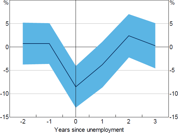
We find that for unemployed workers in our sample, total annual expenditure falls by 9 per cent in the year that the household head is unemployed (Figure 9).^[11] Our estimated effect of unemployment is very similar to estimates for the United States and Sweden of 10 per cent and 13 per cent, respectively (Christelis et al 2015; Landais and Spinnewijn 2019).

Figure 9: Effect of Unemployment on Annual Total Spending

Model estimates

We also test whether the estimated consumption response is due to observable life events that may be correlated both with unemployment propensity and income (and thus consumption). Namely, we test whether educational attainment, change in contract type or industry of work account for the observed consumption response. But including these controls does little to affect the size or statistical significance of our estimates (see Table B1).^[12]

Total consumption takes 2 years to return to pre-unemployment levels, which could be due to persistent income losses (as documented in Lancaster (forthcoming)). In conjunction with Lancaster's estimates of incomes losses, these results show that unemployment leads to larger falls in income than consumption, consistent with consumption smoothing.

However, these estimates may not provide a full picture of consumption losses during unemployment (k = 0) as they do not necessarily capture the contemporaneous effects of unemployment on spending. For instance, a worker may have been unemployed for a few weeks at the time of the survey and is being asked about their spending over the past 12 months, so their spending estimates will be affected by a period of employment. This timing issue matters for identifying the causal effect of unemployment. From a welfare perspective, it can matter too because a sharp decline in spending over a short period of time is different to the same decline in spending spread over a year.

To account for this we conduct the same event study but with higher frequency (weekly) measures of spending. Here, we focus on food spending measures – groceries and eating out – to account for both essential and discretionary spending. Following the same model as before, we estimate the effect of unemployment on weekly grocery spending:

(2)

\ln (g r o c e r i e s_{i t}) = β_{k} \sqrt{n_{i t}} + α_{i} + γ_{t k} + δ_{k} U_{i t - k} + ε_{i t}, \forall k \in {- 2, - 1, ..., 3}

And we estimate the effect of unemployment on weekly eating out expenditure as:

(3)

\ln (e a t i n g o u t_{i t} + \sqrt{e a t i n g o u t_{i t}^{2} + 1}) = β_{k} \sqrt{n_{i t}} + α_{i} + γ_{t k} + δ_{k} U_{i t - k} + ε_{i t k}, \forall k \in {- 2, - 1, ....3}

Here, the model is estimated using the inverse hyperbolic sine function rather than the natural log because households may spend nothing on eating out. In this case, the natural log specification may understate the effect of unemployment on discretionary expenditure (Burbidge, Magee and Robb 1988).

We also consider the effect of unemployment on expenditure on housing (rent and mortgage repayments), as these items are also recorded on a weekly basis:

(4)

\ln (h o u s i n g_{i t} + \sqrt{h o u s i n g_{i t}^{2} + 1}) = β_{k} \sqrt{n_{i t}} + α_{i} + γ_{t k} + δ_{k} U_{i t - k} + ε_{i t k}, \forall k \in {- 2, - 1, ....3}

where housing_it is total household expenditure on rent, mortgage repayments or both.

Since the $δ_{k}$ coefficients denote the effect of unemployment at the time of the survey, these estimates approximate the contemporaneous effect of unemployment on spending.^[13] To again determine how much of the spending response is explained by the contemporaneous fall in income, we also estimate the model including controls for weekly household wage income, and plot these estimates alongside the baseline estimates.^[14]

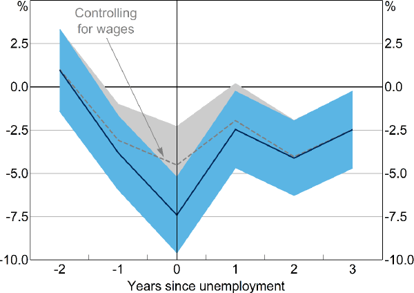
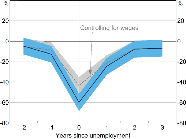
At unemployment, households spend on average 7 per cent less on groceries than similar employed households (Figure 10). The effect on eating out is much greater, with spending falling by 43 per cent (Figure 11). These estimates are in line with previous research that reports average declines in food spending of between 6 and 10 per cent in response to unemployment (Gruber 1997; Chetty and Szeidl 2007; Hendren 2017). After controlling for household wages, the fall in grocery expenditure is smaller, but still statistically significant at 2.5 per cent. Similarly, a fall in expenditure on meals eaten outside the home persists after controlling for household wages, but remains large at around 30 per cent. This may be because households substitute away from eating out and cook more at home as the opportunity cost of doing so falls (Aguiar and Hurst 2005).

Figure 10: Effect of Unemployment on Grocery Spending

Model estimates

Figure 11: Effect of Unemployment on Spending on Meals Outside the Home

Model estimates

The effect on both types of spending persists 3 years after unemployment, even after controlling for income losses. This finding is consistent with literature that finds that unemployment leads to persistent changes in spending habits. For instance, households with members that have lived through high unemployment are more likely to buy lower-end products (Malmendier and Shen 2021). Alternately, this could suggest that households take some time to rebuild lost savings buffers following an unemployment spell. Consistent with Hendren (2017), we find a significant fall in food spending in the year before unemployment. Unlike Hendren, we find this fall in spending is largely explained by lower wage income, which is likely due to reduced hours worked in the lead-up to unemployment (Lancaster forthcoming).

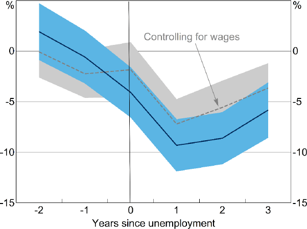
Unemployment also has a significant effect on housing expenditure. Households reduce their spending on their home in the year of unemployment, with spending remaining low for at least the next 3 years, even after wages recover.^[15] This again could reflect some household consumption decisions, such as housing, being ‘committed’, or could reflect that households reduce expenditure on housing in order to rebuild savings buffers following unemployment.^[16]

Figure 12: Effect of Unemployment on Housing Spending

Model estimates

Footnotes

See Meyer and Sullivan (2003) for further discussion of economic measures of wellbeing. [6]

Gruber (1997), Browning and Crossley (2001), Chetty and Szeidl (2007) and Christelis et al (2015) estimate consumption losses from unemployment in the United States, and Landais and Spinnewijn (2019) does the same for Sweden. [7]

See Salant (1977) for more information on length-biased sampling and the implications for unemployment data. [8]

The household ‘head’ is identified in the HILDA Survey by applying the following criteria, in order, until a unique person is selected. The criteria are: i) a registered or de facto marriage; ii) a long parent; iii) the person with the highest financial year income; and iv) the eldest person. We use the household head status in the previous year as the head selection criteria. [9]

See Krolikowski (2017) for a discussion of the problems associated with estimating causal effects of unemployment. [10]

If other household members increase their hours in response to unemployment of the head, these estimates may be understated. However, the literature finds little empirical support for this (Cullen and Gruber 2000). It is also likely that consumption effects are larger for single-income families than those presented here. [11]

Specifically, the controls are the age and education level of the household head, contract type (e.g. permanent, casual or fixed term) and industry of work. We also re-estimate all specifications in first differences and find no substantive differences in our results. [12]

The survey respondents are asked to report spending in ‘a normal week’, which could be interpreted as the period before unemployment. As a result, while the results are similar to the literature, it is possible that the estimates are understated. [13]

We use the inverse hyperbolic sine of weekly wages of the entire household. [14]

When income returns to levels comparable with households that had never experienced unemployment, the dashed lines and solid lines meet in Figures 10 through 12, indicating income plays no explanatory role. [15]

While we only consider wage income in these specifications, the fall in total income (including public transfers) would explain even less of the observed fall in expenditure at unemployment. This is because public transfers rise during unemployment. [16]