Research Discussion Paper – RDP 2021-08 Job Loss, Subjective Expectations and Household Spending
1. Introduction
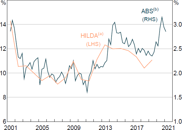
Job insecurity (or ‘job loss risk’) is a key uncertainty that workers face, particularly during recessions. Elevated levels of job insecurity have been a feature of the economic downturn associated with the COVID-19 pandemic (Figure 1). The extent to which job insecurity persists and affects household spending is important to determining the sustainability of the post-pandemic economic recovery.
Notes:
(a) Average reported chance of involuntary job loss over the next 12 months
(b) Per cent of employed persons not expecting to be with current employer in 12 months due to involuntary job loss
Sources: ABS: HILDA Survey Release 19.0
It is well-established that job loss is associated with reductions in earning and spending for workers.[1] But there are many things we do not know about the links between workers' perceptions of their job prospects, actual job outcomes and spending. For example, do workers expect to lose their jobs? How long do the unemployed expect to be without a job? And do these expectations affect household spending behaviour?
Standard consumption theories, such as the permanent income hypothesis (PIH), posit that consumers choose a steady level of consumption in line with their expectations of total lifetime earnings. Under the PIH, households adjust their spending in response to unexpected changes in current income and to changes in their expectations of future income. This implies that households should adjust their spending by more in response to job loss events that are unexpected and/or convey new information about their future job prospects. This suggests that households' subjective beliefs about their current and future income matter to their spending decisions.
In this paper we test these ideas and make several contributions to the literature on job loss, subjective expectations and household spending.
First, we document some stylised facts about subjective expectations regarding future job outcomes. We confirm previous findings that workers have some ability to predict job loss a year ahead, even when controlling for a range of personal characteristics, suggesting that they hold some private information about their future prospects (Dickerson and Green 2012; McGuinness, Wooden and Hahn 2014).
Second, we extend these insights by showing that there are systematic differences between workers' predictions for job loss in the year ahead and actual (ex post) outcomes (we refer to these differences as ‘forecast deviations’). Specifically, there is an intrinsic time-invariant component (or ‘fixed effect’) to workers' expectations of job loss. Most workers persistently overestimate their job loss risk, but some persistently underestimate it.
Third, we show that these job loss forecast deviations co-move with the business cycle – the average worker typically overestimates the probability of job loss by more during economic downturns. And there is a structural component to forecast deviations too – the extent to which workers systematically overestimate the probability of job loss has increased since 2013. This is consistent with elevated job insecurity, lower worker bargaining power and weak wages growth during this time (Foster and Guttmann 2018).
Fourth, we find that individuals' expectations for the duration of unemployment have some predictive power for the actual duration. While workers are overly pessimistic about losing their jobs, the unemployed are too optimistic about finding a job (Mueller, Spinnewijn and Topa 2021).
To the best of our knowledge, these behavioural insights of systematic bias amongst workers are new to the literature. Taken together, these results point to clear violations of standard models of expectation formation, such as the full information rational expectations model. These systematic biases also have implications for job matching and, more generally, household spending behaviour.
We then explore the links between job loss, expectations and spending. We find that the typical household reduces spending by 9 per cent in the year of unemployment. Spending losses are not limited to discretionary spending, with grocery expenditure falling by 7 per cent at unemployment. These consumption losses also extend to the period after unemployment, and are smaller but still exist even when accounting for income losses. These findings suggest that household spending is excessively sensitive to predictable changes in income, which is consistent with previous empirical work (e.g. Gruber 1997; Ganong and Noel 2019) but inconsistent with standard workhorse models, such as the PIH. We find only limited evidence that concerns about future job loss affect spending for those workers that do not actually lose their jobs.
It is well established that unemployment is associated with significant welfare losses (Gruber 1997). Our research goes some way to quantifying the effect on welfare by documenting the size (and persistence) of consumption losses associated with unemployment. For policymakers, our results highlight the costliness of unemployment to households and reaffirm the importance of policies that keep the level and duration of unemployment low.
2. Measuring Subjective Employment Expectations and Household Spending
2.1 Subjective employment expectations
The analysis in this paper relies on household-level data sourced from the Household, Income and Labour Dynamics in Australia (HILDA) Survey. The HILDA Survey is a longitudinal study that tracks a representative sample of more than 17,000 individuals from 2001 to 2019. The panel nature of the HILDA Survey allows us to exploit heterogeneity in household spending patterns and labour market outcomes while controlling for individual time-invariant characteristics.
The HILDA Survey asks employed respondents about their subjective employment expectations. Specifically, respondents are asked the following question on the subjective probability of job loss:
What do you think is the per cent chance that you will lose your job during the next 12 months? (That is, get retrenched or fired or not have your contract renewed.)
Responses are given as integer values from 0 to 100 where 0 indicates no chance, and 100 absolute certainty. We use this probabilistic response as our measure of individuals' subjective probability of job loss.
Looking at the distribution of job loss probabilities, there is clear ‘bunching’ in responses at 0, 50 and 100 per cent (Figure 2). This distribution is commonly observed in studies of subjective job loss expectations (Manski and Straub 2000; Stephens 2004). The bunching is at least partly due to respondents rounding their answers (Kleinjans and van Stoest 2010).
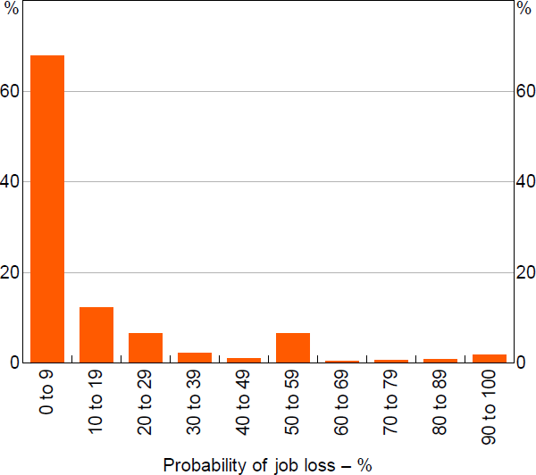
Note: Employment terminated or contract not renewed
Sources: Authors' calculations; HILDA Survey Release 19.0
Similar to the variable on job loss expectations, individuals who are not employed but are looking for work are asked the following question on the probability of finding suitable employment:
What do you think is the per cent chance that you will find a suitable job during the next 12 months?
Again responses range from 0 to 100 where 0 indicates no chance, and 100 absolute certainty. We take this variable as our measure of unemployed individuals' subjective probabilities of finding a job.
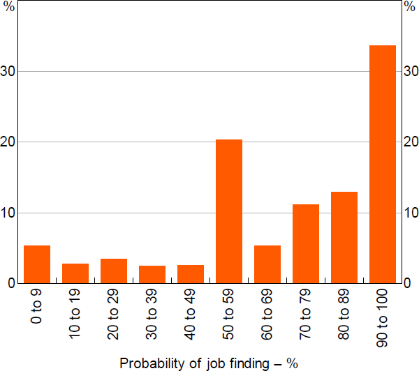
The distribution of the unemployment duration variable also displays evidence of bunching, particularly at 50 per cent (Figure 3). The implied distribution suggests that most unemployed persons expect to find work within a year. But there is considerable dispersion among individuals' expectations of the duration of unemployment.
Sources: Authors' calculations; HILDA Survey Release 19.0
We are able to examine the realisation of job loss events by using the response to the question:
Did any of these (events) happen to you in the past 12 months … fired or made redundant by an employer?
Given households are surveyed every 12 months, the response to this question corresponds perfectly with the wording in the expectations of job loss question. This allows us to closely explore the links between expected and actual job outcomes.
2.2 Household spending
The HILDA Survey collects detailed information on household spending each year. This includes spending on non-durable goods and services (for the years 2006 to 2019) and durable goods (for a limited sample window between 2006 and 2010).
To measure different types of spending, survey respondents are asked to complete a questionnaire. Respondents are first asked if they have any responsibility for the payment of household bills (such as household groceries, electricity, gas and water). If so, respondents are then directed to the following question:
For each type of expenditure below, write in your best estimate of the total amount spent on that item by all people in the household.
Respondents fill out expenditure amounts for a list of items, and are asked to report how much they spent on each item in the last 12 months. Our measure of annual expenditure comes from aggregating these items, as shown in Table 1. For weekly expenditure, respondents are asked to report how much they spend on each item per week on average. Weekly expenditure is recorded for a limited number of items, as shown in Table 1.
| Non-durables (2006 to 2019) | Durables (2006 to 2010) | |
|---|---|---|
| Annual | Groceries | Motor vehicles (new and used) |
| Meals eaten out | Computers and related devices | |
| Alcohol and tobacco | Audio visual equipment | |
| Transport | Household appliances | |
| Holiday travel | Furniture | |
| Clothing and footwear | ||
| Motor vehicle fuel and maintenance | ||
| Home repairs, renovation and maintenance | ||
| Healthcare fees and products | ||
| Utilities | ||
| Telecommunications | ||
| Education fees | ||
| Insurance | ||
| Weekly | Groceries | |
| Meals eaten out | ||
|
Source: HILDA Survey Release 19.0 |
||
We mainly focus on food spending (including groceries and meals eaten out) for a few reasons.[2] First, food expenditure is one of the few survey items that is recorded on a weekly basis. Using weekly expenditure should give more insight into the contemporaneous effects of job loss on spending. For example, a small decline in annual spending in the year of job loss would not tell us if the household reduced spending a little but spread it out over the full year, or if they reduced spending a lot for a short period of time. These 2 possibilities have different implications for the welfare effects of unemployment. Second, food expenditure has been shown to suffer from less measurement error than other spending categories in survey data.[3] Third, food expenditure, particularly groceries, is also commonly used in existing research, making it easier to compare our results to the literature. Food spending can also be disaggregated into grocery expenditure and expenditure on meals eaten outside of the home. This split can offer some insight into how the response of more essential expenditure (groceries) compares to the response of discretionary spending (meals outside of the home).
The HILDA Survey also contains information on household income and wealth. These variables are partly used as controls in the model estimation but are also used to explore the heterogeneous effects of job loss on household spending. Household income data is available for every sample year, but wealth data are available only every 4 years from 2002 and 2018.
3. Can Workers Predict Actual Labour Market Outcomes?
3.1 Do employed workers expect to lose their jobs?
In this section, we confirm some previous research findings about worker expectations for job loss. First, we find workers typically overestimate the probability of job loss (Figure 4). This finding holds at all levels of job loss expectations, as evidenced by the actual rate of job loss being persistently below the estimated probability of job loss. While it is possible that workers may voluntarily resign in anticipation of job loss, we find that this does not explain the discrepancy, with expected job loss remaining higher than the rate of job separation on average, regardless of whether the worker voluntarily left the job or not. Expectations of job loss do appear to contain some predictive information, as they increase with the actual probability of job loss. However, the difference between estimated and actual job loss also increases with job loss expectations.
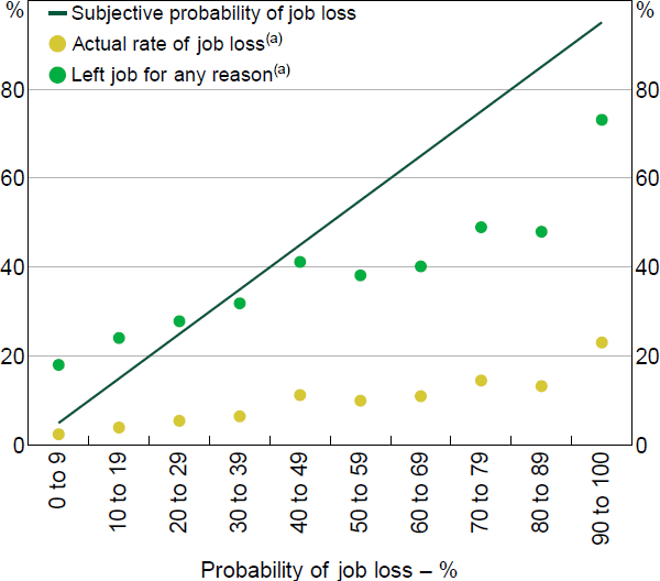
Note: (a) Subjective probability of losing job as reported by respondent in the previous year
Sources: Authors' calculations; HILDA Survey Release 19.0
In Appendix A, we outline a simple model of expectations formation to more formally test the predictive ability of workers' subjective expectations. In particular, we adapt the framework of Keane and Runkle (1990) to examine whether worker expectations are fully rational, or whether their mistakes are systematic and predictable and should be accounted for when forming expectations.
The results shown in Appendix A indicate that workers have some ability to predict actual job loss in the year ahead. Indeed, subjective job loss expectations contain predictive power over and above the observed characteristics of the worker at the time of the survey. A 1 percentage point increase in the expected probability of job loss is associated with an increase of about 10 to 18 basis points in the actual probability of job loss.
But here we focus on evidence of systematic bias in forecasting future job prospects. For this, we follow a 2-stage process. First, we estimate a simple model of the ‘objective’ (or ‘true’) probability of job loss for each worker based on their own characteristics, including private information that is not observed by the researcher. Second, we compare this model-based probability estimate to the worker's subjective estimate. We then look for evidence of systematic deviations between the model-based and subjective estimates, both across workers and over time.
First, the objective probability of job loss is assumed to be given by the following model:
Which states that the worker's latent probability of job loss is a function of various personal characteristics that are observed by the researcher ( xit ), such as age, job tenure and industry of work, as well as a subset of characteristics that only the worker observes as private information . In practice, actual job loss (yit+1) is observed as a binary outcome, as shown by the indicator function, I (A), that is equal to one if the statement, A, is true and is zero otherwise.
This model is estimated using a logistic regression. The observed job loss outcome is assumed to be a function of both worker characteristics observed by the researcher as well as the worker's private information, which is assumed to be captured by their subjective belief :
The predictions from the logistic regression are our proxy for the model-based or ‘objective’ probability estimates .
Second, to construct estimates of forecast deviations we take the difference between the worker's subjective belief and the model-based probability estimates:
This forecast deviation is assumed to be a function of a worker fixed effect , a year fixed effect and a white noise error term (vit+1). The worker fixed effect captures the systematic ability or willingness of each worker to forecast their job market prospects a year ahead. This persistent cross-sectional variation could reflect several unobserved factors. For example, it may be due to differences in forecasting ability (e.g. economic literacy), effort or optimism.
The distribution of the estimated worker fixed effects indicates that most workers display a positive bias in that they persistently overestimate the probability of job loss, but there are some workers that persistently underestimate it (Figure 5).
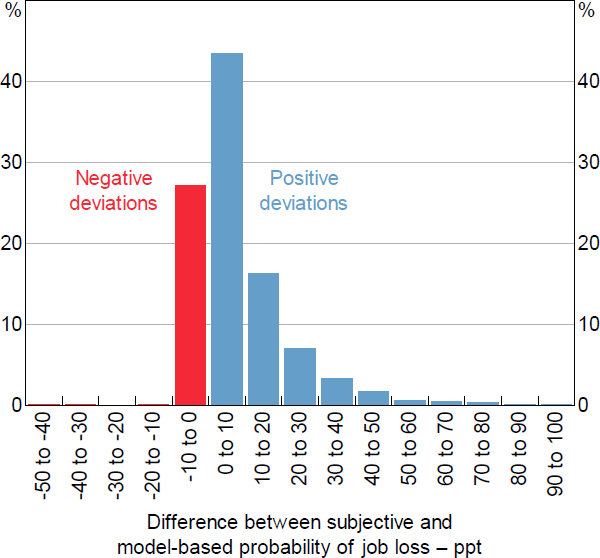
Notes: Forecast deviations are estimated as worker fixed effects from a panel regression of the difference between the subjective estimate and the model-based estimate of job loss; the regression also includes year fixed effects
Sources: Authors' calculations; HILDA Survey Release 19.0
The average worker not only overestimates the probability of job loss, but the extent of this overestimation varies with aggregate labour market conditions, as shown by the time fixed effects (Figure 6). Expectations of job loss for the average worker rose by more than the model-based probability estimates during both the economic downturn in 2001 and the global financial crisis (GFC). And, since around 2013, the difference between the expected and model-based outcomes has increased compared to the period before the GFC, alongside elevated levels of job insecurity during that time (Foster and Guttmann 2018).
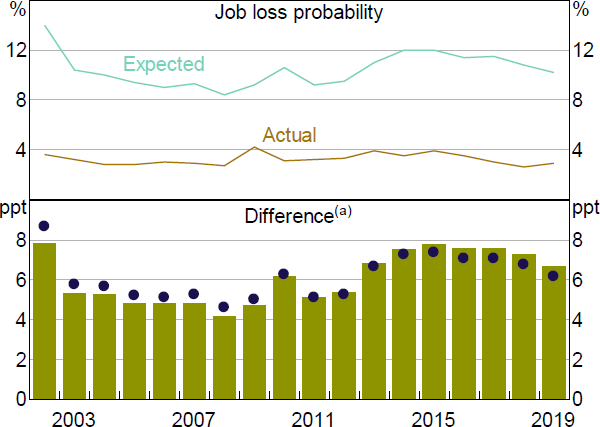
Note: (a) The bars represent the average difference between the subjective and model-based estimates of job loss, while the dots represent the estimated year fixed effects
Sources: Authors' calculations; HILDA Survey Release 19.0
3.2 Do unemployed workers expect to find a job?
Next, we focus on workers that are unemployed and explore the ability of their subjective expectations to predict finding a suitable job in the year ahead. This allows us to examine expectations of the duration of unemployment, which could be relevant to household spending.
The data indicate that unemployed workers typically overestimate the probability of finding a job (Figure 7). But workers that believe they have little chance of finding a job actually understate the probability of job finding. This indicates that the expectations of both employed and unemployed workers deviate from actual future labour market outcomes, on average. However, expected job finding rates do increase with actual rates, which is consistent with prior research (Spinnewijn 2015; Mueller et al 2021). More formal tests of the predictive ability of the subjective expectations of unemployed workers can be found in Appendix A.
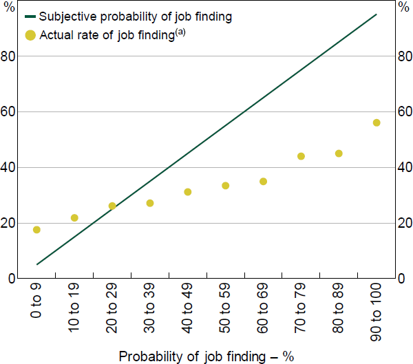
Note: (a) Subjective probability of finding job reported by respondent in the previous year
Sources: Authors' calculations; HILDA Survey Release 19.0
Given the longitudinal nature of the survey, we can also examine how expectations of job finding evolve during a spell of unemployment. We find that expectations of job finding are lower the longer a worker has been unemployed (Figure 8). There are two competing explanations for this observed relationship, as discussed by Mueller et al (2021). The negative relationship between job finding expectations and duration could represent ‘true’ duration dependence, whereby unemployed respondents become increasingly discouraged the longer they are unemployed and revise down their expectations of job finding. Alternately the relationship may be due to ‘dynamic selection’, in which there is a shift in the composition of the pool of unemployed. Under dynamic selection, respondents with lower expectations of job finding remain unemployed for longer, leading to the observed relationship between unemployment duration and job finding expectations.
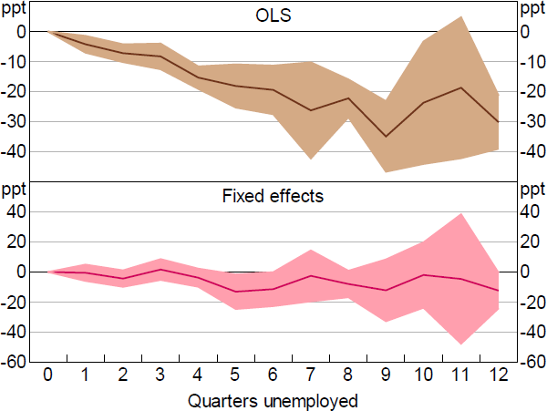
Notes: Base category = < 1 quarter; shaded areas are 95 per cent confidence intervals
Sources: Authors' calculations; HILDA Survey Release 19.0
We can distinguish whether the decline in expected job finding probability is due to either of these explanations by exploiting the longitudinal nature of the household survey data. If there is true duration dependence in expectations of job finding, we should observe a decline in the expected probability of job loss for a worker in a given spell of unemployment (a within-worker effect). If there is dynamic selection we should observe a decline in the expected probability of job loss across spells for different workers (a between-worker effect) (Mueller et al 2021).
To disentangle these competing explanations we estimate a regression for unemployed workers in which the dependent variable is the expected probability of finding a job and the explanatory variables are a vector of dummies for time spent unemployed (in years). By comparing the regression estimates with and without a worker fixed effect, we can gauge how expected job finding probability evolves within and between unemployed workers.
We find that the expected job finding rate declines with the length of the unemployment spell, but that this effect disappears once we include a worker fixed effect (Figure 8). This indicates that the decline in the expected probability of job finding is due to the dynamic selection effect, with a gradual shift over the duration of unemployment towards unemployed workers with lower expected probabilities of finding jobs.[4]
3.3 Why are there differences between actual and expected job outcomes?
The systematic differences between expected and actual job outcomes could be explained by a range of factors that vary across workers, such as forecasting ability, effort or degree of optimism.
We do not pin down the mechanism that explains these differences across workers, though we provide some tentative evidence suggesting that optimism could be part of the story. Specifically, we find that workers that overestimate their probability of job loss are more likely to underestimate their probability of job finding, on average. This is based on the observation that there is a (small) negative correlation between the worker fixed effects for the rate of job loss and job finding. This could be taken as evidence that some workers are too pessimistic about their future job prospects.
However, the observed overestimates of job loss rates and underestimates of job finding rates could also be explained by ‘conservatism’ in perceptions of probability (Khaw, Stevens and Woodford 2021). Conservatism refers to the observation that individuals tend to overstate low probability events (such as losing your job), and understate high probability events (such as keeping your job). This phenomenon has been identified under numerous settings in the experimental psychology literature, but we have not seen it applied to subjective labour market expectations (Attneave 1953; Varey, Mellers and Birnbaum 1990).[5]
We leave a more complete investigation of the mechanisms that explain these systematic deviations to future research. However, it is worth noting that predicting your future job prospects is generally a very challenging task. For instance, in estimating their probability of job loss, a worker needs to make predictions about a range of factors that are outside their control, including forecasting how economic conditions will evolve over the coming year, understanding how changes in economic conditions will affect their own firm, and subsequently predicting how much they are at risk of losing their job. In doing so, the worker may not correctly estimate the consequences of the change in economic conditions, or how the shock is distributed across firms, or how their specific job will be affected. Misspecification at any one of these points can lead to measured differences between subjective and objective (model-based) probabilities.
Moreover, an employed worker can influence their own objective probability of job loss. For example, workers that expect to lose their job have an incentive to find another job and quit before they involuntarily lose their job. This will reduce the actual probability of job loss relative to the subjective estimate (and lead to a larger positive deviation). This selection effect is partly captured by the measured difference between the subjective and objective probability of job loss shown in Figure 4. Alternatively, workers that expect to lose their job may have a greater incentive to work harder to keep it. The additional work effort may lower the actual probability of job loss relative to their subjective estimate (leading to a larger negative deviation). If individuals most at risk work harder to improve their value to the firm, the firm has less incentive to make them unemployed involuntarily.
4. How Does Unemployment Affect Household Spending?
The next part of the paper explores the effects of unemployment, and expectations of job loss, on household spending. Understanding the relationship between household-level consumption, expectations and unemployment can shed light on how households make economic decisions, and test various theories of household consumption. While we have previously considered job loss, we now consider unemployment. This is primarily because the HILDA Survey asks about typical or current expenditure, meaning we are unable to observe consumption losses from unemployment spells that occur because of job losses between survey waves. To get around this, we focus only on workers who are unemployed as at the time of the survey. Despite this, we acknowledge that in some circumstances a job loss event may not be followed by unemployment (if the worker leaves the labour force, or finds new employment immediately), and in others unemployment may not be the result of job loss (if an unemployed respondent voluntarily left their previous job, for example).
In addition, the consumption response to unemployment may help us quantify the welfare effects of unemployment on households. Unlike current income, consumption relates directly to household welfare. This is because temporary fluctuations in income may be smoothed over the life cycle, while consumption is typically less volatile. To the extent that we want to capture the effect of unemployment on economic wellbeing, consumption is a better indicator.[6]
4.1 Theoretical framework
To frame the analysis that follows it is useful to outline how household consumption responds to changes in income under the assumptions of a standard workhorse model, such as the PIH (Stephens 2004; Been et al 2020). In this set-up, households are assumed to be infinitely lived, face constant interest rates, have quadratic utility functions and supply labour perfectly elastically. The only source of uncertainty in the model is about future income. Under these assumptions, optimal consumption can be expressed as:
where Cit denotes consumption of household i at time t, r is the constant interest rate, Yit denotes income and Wit is total wealth. It follows that the growth rate of household spending can be written:
This equation shows that there are two parts to the contemporaneous effect of income changes on household spending. The first term on the right-hand side of the equation shows that changes in income only have a contemporaneous effect on spending if they are unexpected. The second term shows that changes in expectations of future income will result in a change in consumption. Changes in contemporaneous income will affect expected future income if households expect the income change to be persistent. If so, a household will adjust their spending by more to take into account this new information. In summary, changes in income will have the strongest contemporaneous effect on spending when they are unexpected and persistent. We test these ideas by looking at whether job loss expectations affect the sensitivity of household spending to unemployment.
4.2 The effect of actual unemployment on household spending
To test the consumption response to unemployment, we estimate a series of reduced form regressions. There is a reasonably large body of research that studies the links between unemployment and consumption.[7] To our knowledge, we are the first to provide Australian estimates of the consumption response to unemployment at the household level. Some care should be taken in interpreting our results – the nature of using survey data means that we are only able to make inferences about the consumption response of the pool of the unemployed at a single point in time in any given survey year. A worker is more likely to appear to be unemployed in a cross-sectional survey the longer they are actually unemployed. This means that the results may not be informative about a typical unemployment spell because longer spells are over-represented. This could lead to biased estimates if the consumption response to unemployment varies with the duration of unemployment.[8] We discuss this potential bias in more detail in Section 6.
We adopt an event study approach and estimate a series of regressions to identify the effects of unemployment on spending. Specifically, we examine how consumption evolves around an unemployment event in the following set-up:
where Cit is household i's annual expenditure in year t ; nit is the number of members in household i in year t , is a vector of year dummies, Uit–k is an indicator for unemployment of the household head at the time of the survey in year t – k, is the error term and is a household fixed effect. The index t here refers to any year in which the person who was the household head in the previous year is observed as unemployed.[9] The fixed effects fully control for household characteristics that do not vary over time and may be correlated with either spending or the risk of unemployment. This could include factors like household preferences, risk aversion and worker ability. We exclude household heads that are not in the labour force from the sample, as we are interested in the spending response to unemployment, relative to spending in employment.
The coefficient of interest, , is the estimated log difference in spending in period t between those that lose their job in period t – k and those that do not. This coefficient can be interpreted as the per cent change in spending due to unemployment (once we multiply by 100). By running separate regressions for all , we produce and plot a series of estimated which show how spending evolves before, during, and after a job loss event.
This method estimates the effect of unemployment in year t on spending in other years. We do not control for unemployment status in years t – k where . That is, the estimates allow current unemployment to affect future consumption through a correlation with future unemployment. This feature, alongside the household fixed effects, helps to capture the causal effects of unemployment.[10]
We find that for unemployed workers in our sample, total annual expenditure falls by 9 per cent in the year that the household head is unemployed (Figure 9).[11] Our estimated effect of unemployment is very similar to estimates for the United States and Sweden of 10 per cent and 13 per cent, respectively (Christelis et al 2015; Landais and Spinnewijn 2019).
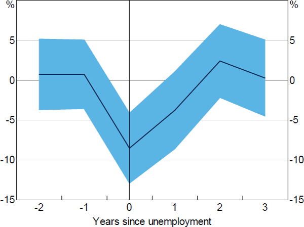
Notes: Coefficients from separate regressions of leads and lags of an indicator of unemployment on the log of annual total expenditure, with controls for year and individual fixed effects and number of persons in household; shaded area is 95 per cent confidence interval with clustered standard errors
Sources: Authors' calculations; HILDA Survey Release 19.0
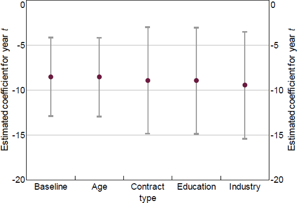
We also test whether the estimated consumption response is due to observable life events that may be correlated both with unemployment propensity and income (and thus consumption). Namely, we test whether educational attainment, change in contract type or industry of work account for the observed consumption response. But including these controls does little to affect the size or statistical significance of our estimates (see Table B1).[12]
Total consumption takes 2 years to return to pre-unemployment levels, which could be due to persistent income losses (as documented in Lancaster (forthcoming)). In conjunction with Lancaster's estimates of incomes losses, these results show that unemployment leads to larger falls in income than consumption, consistent with consumption smoothing.
However, these estimates may not provide a full picture of consumption losses during unemployment (k = 0) as they do not necessarily capture the contemporaneous effects of unemployment on spending. For instance, a worker may have been unemployed for a few weeks at the time of the survey and is being asked about their spending over the past 12 months, so their spending estimates will be affected by a period of employment. This timing issue matters for identifying the causal effect of unemployment. From a welfare perspective, it can matter too because a sharp decline in spending over a short period of time is different to the same decline in spending spread over a year.
To account for this we conduct the same event study but with higher frequency (weekly) measures of spending. Here, we focus on food spending measures – groceries and eating out – to account for both essential and discretionary spending. Following the same model as before, we estimate the effect of unemployment on weekly grocery spending:
And we estimate the effect of unemployment on weekly eating out expenditure as:
Here, the model is estimated using the inverse hyperbolic sine function rather than the natural log because households may spend nothing on eating out. In this case, the natural log specification may understate the effect of unemployment on discretionary expenditure (Burbidge, Magee and Robb 1988).
We also consider the effect of unemployment on expenditure on housing (rent and mortgage repayments), as these items are also recorded on a weekly basis:
where housingit is total household expenditure on rent, mortgage repayments or both.
Since the coefficients denote the effect of unemployment at the time of the survey, these estimates approximate the contemporaneous effect of unemployment on spending.[13] To again determine how much of the spending response is explained by the contemporaneous fall in income, we also estimate the model including controls for weekly household wage income, and plot these estimates alongside the baseline estimates.[14]
At unemployment, households spend on average 7 per cent less on groceries than similar employed households (Figure 10). The effect on eating out is much greater, with spending falling by 43 per cent (Figure 11). These estimates are in line with previous research that reports average declines in food spending of between 6 and 10 per cent in response to unemployment (Gruber 1997; Chetty and Szeidl 2007; Hendren 2017). After controlling for household wages, the fall in grocery expenditure is smaller, but still statistically significant at 2.5 per cent. Similarly, a fall in expenditure on meals eaten outside the home persists after controlling for household wages, but remains large at around 30 per cent. This may be because households substitute away from eating out and cook more at home as the opportunity cost of doing so falls (Aguiar and Hurst 2005).
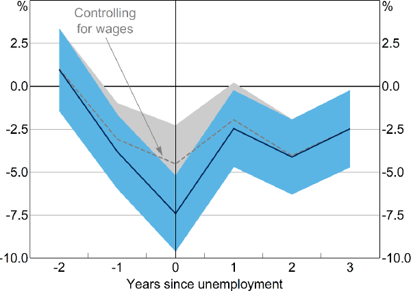
Notes: Coefficients from separate regressions of leads and lags of an indicator of unemployment on the log of weekly grocery expenditure, with controls for year and individual fixed effects and number of persons in household; shaded areas are 95 per cent confidence intervals with clustered standard errors
Sources: Authors' calculations; HILDA Survey Release 19.0
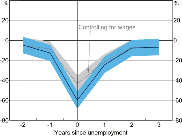
Notes: Coefficients from separate regressions of leads and lags of an indicator of unemployment on the inverse hyperbolic sine of weekly household expenditure on meals outside the home, with controls for year and individual fixed effects and number of persons in household; shaded areas are 95 per cent confidence intervals with clustered standard errors
Sources: Authors' calculations; HILDA Survey Release 19.0
The effect on both types of spending persists 3 years after unemployment, even after controlling for income losses. This finding is consistent with literature that finds that unemployment leads to persistent changes in spending habits. For instance, households with members that have lived through high unemployment are more likely to buy lower-end products (Malmendier and Shen 2021). Alternately, this could suggest that households take some time to rebuild lost savings buffers following an unemployment spell. Consistent with Hendren (2017), we find a significant fall in food spending in the year before unemployment. Unlike Hendren, we find this fall in spending is largely explained by lower wage income, which is likely due to reduced hours worked in the lead-up to unemployment (Lancaster forthcoming).
Unemployment also has a significant effect on housing expenditure. Households reduce their spending on their home in the year of unemployment, with spending remaining low for at least the next 3 years, even after wages recover.[15] This again could reflect some household consumption decisions, such as housing, being ‘committed’, or could reflect that households reduce expenditure on housing in order to rebuild savings buffers following unemployment.[16]
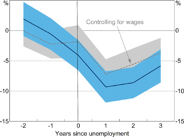
Notes: Coefficients from separate regressions of leads and lags of an indicator of unemployment on the inverse hyperbolic sine of monthly expenditure on rent and mortgage payments, with controls for year and individual fixed effects and number of persons in household; shaded areas are 95 per cent confidence intervals with clustered standard errors
Sources: Authors' calculations; HILDA Survey Release 19.0
5. Do Expectations Affect the Sensitivity of Household Spending to Unemployment?
So far we have documented 2 observations about Australian households. The first is that, as in other countries, individuals are able to foresee both job loss and job finding at least to some extent. The second observation is that at unemployment, households significantly reduce their spending. We now link these 2 findings and explore whether the sensitivity of consumption to unemployment is affected by whether the household expected to lose their job or not.
As shown in Section 4.1, standard consumption models predict that households will mostly adjust spending in response to unexpected shocks to current income. Any adjustment to expected income shocks could be taken as evidence against these theoretical models. We directly test these ideas within the following regression framework:
Equation (5) is specified in the same way as Equations (1) through (4), however here we only consider spending in the year of unemployment. We include the same controls as before but now also add a term for (lagged) job loss expectations of the household head, . This measure ranges from 0 if they perceived no chance of job loss to 1 if they perceived job loss was certain. We also include an interaction term between lagged job loss expectations and a dummy for whether the household head became unemployed during the survey year.
Under this specification, the change in spending in response to unemployment is estimated by . Consider 2 extreme cases. The coefficient captures the effect of unemployment on spending for those working household heads that fully expect to not lose their jobs and hence are completely ‘surprised’ by unemployment. The sum of the coefficients captures the spending response to unemployment in the case in which a working household head fully expects to lose their job and hence is completely unsurprised by unemployment . The coefficient therefore captures how the consumption sensitivity to unemployment varies with job loss expectations.
Within this framework we can also test whether household spending is sensitive to job loss expectations for households that do not lose their jobs. This is captured by the coefficient on the lagged job loss expectations term. This allows us to explore the links between job insecurity and household spending for all households, not just those actually affected by unemployment.
As before, we separately estimate Equation (5) for different types of spending as the dependent variable, including spending on groceries, meals eaten outside the home and all items (including durable goods).
Results for all 3 specifications are presented in Table 2. We find that the fall in spending at unemployment is large for those that are completely surprised by unemployment (as shown by the large negative coefficient, ). This is consistent with the predictions of standard workhorse models. But we also find that the fall in spending at unemployment is just as large when the household at least partly expects job loss (as shown by the negative coefficient on the sum of the coefficients, , and the fact that estimates of are not significantly different from 0). This suggests that households adjust spending in response to a predictable change in income (unemployment), which contradicts the predictions of standard models. However, this result is consistent with prior empirical research suggesting that household spending is excessively sensitive to predictable income changes (Japelli and Pistaferri 2017).
For grocery expenditure, and spending on meals eaten outside the home, we find that lagged job loss probability does not provide any additional information about household expenditure, as shown by the estimates of that are not statistically significantly different from 0. This tells us that households who do not lose their jobs also do not adjust their spending on these expenditure categories when their expectations of job loss change. However, we find our estimate of to be significant and negative in the regression with total annual expenditure. The coefficient estimate of -0.04 means that households that change their probability of job loss from 0 (no chance) to 1 (100 per cent certainty) decrease their total spending in the following year by 4 per cent. This result provides some suggestive evidence that job security may matter for spending on some goods and services.
| Dependent variable | Groceries | Meals eaten outside the home | Total expenditure |
|---|---|---|---|
| Unemployed | −0.05*** (0.01) |
−0.44*** (0.05) |
−0.05* (0.03) |
| Unemployed * lagged job loss probability | −0.03 (0.04) |
0.11 (0.15) |
−0.02 (0.07) |
| Lagged job loss probability | 0.01 (0.01) |
−0.03 (0.02) |
−0.04** (0.02) |
| Fixed effects | Yes | Yes | Yes |
| R squared (overall) | 0.31 | 0.01 | 0.16 |
| Observations | 96,060 | 91,461 | 30,558 |
|
Notes: ***, ** and * denote statistical significance at the 1, 5 and 10 per cent levels, respectively; standard errors in parentheses; coefficient estimate for year dummies and number of persons in household omitted Sources: Authors' calculations; HILDA Survey Release 19.0 |
|||
6. Why Does Unemployment Reduce Spending
Next, we identify heterogeneity across households in the spending response to unemployment. This heterogeneity allows us to explore further the mechanisms through which job loss affects spending.[17] We also further explore the role of worker beliefs in determining the size of the effect of job loss on spending.[18] We focus on weekly food spending and test various violations of the PIH which might explain the unemployment effect found in Section 5:
- Liquidity constraints: if the effect is due to liquidity constraints then we should find stronger spending responses to unemployment for those individuals that are estimated to be liquidity constrained (or ‘hand-to-mouth’), and we should see no effect until unemployment occurs.
- Myopia: if individuals are short-sighted then we should see no spending response until actual unemployment occurs, and the effect should be stronger for households that reportedly do not plan ahead in terms of their saving and spending decisions.
- Precautionary saving: if households expect to remain unemployed for longer, they may reduce their expenditure in unemployment by more in order to smooth consumption over the unemployment spell.
We explore these forms of heterogeneity through the same event study framework as before, but we now run separate sub-sample regressions for different types of households and/or different unemployment events:
where the model specification is as before, but we now include an indicator for whether the household head is, for example, hand-to-mouth (j = 1) and compare to the case in which the household head is not hand-to-mouth (j = 0) in in the year before unemployment based on 2 different regressions. We again also estimate the model with the log of total spending as the dependent variable for comparison.[19]
To test for liquidity constraints, we identify households that are liquidity constrained based on the framework developed by Kaplan, Violante and Weidner (2014). Under this approach, households may be sensitive to shocks to current income despite relatively high levels of wealth (because many households hold wealth in relatively illiquid assets, such as housing and superannuation).[20]
For this, we estimate the model separately for liquidity-constrained households and all other households. We find that liquidity-constrained households reduce spending by more than other households in response to unemployment (Figure 13). Interestingly, liquidity-constrained households also reduce spending in the year before unemployment. This is consistent with liquidity constraints being an important part of the story. It also highlights that even asset-rich households may experience large consumption losses due to illiquid wealth. Households that are not liquidity constrained also reduce spending in response to unemployment.
We follow the same sub-sampling approach to test whether myopic households are more sensitive to unemployment in their spending response. We measure myopia based on responses to a specific question about the time frame in which each household plans saving and spending decisions. A household is considered myopic if the most important time frame is one year or less. On this metric, we find no difference between the spending responses at the onset of unemployment for myopic households compared to forward-looking households (Figures 14 and 15).
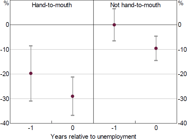
Note: Lines represent 95 per cent confidence intervals
Sources: Authors' calculations; HILDA Survey Release 19.0
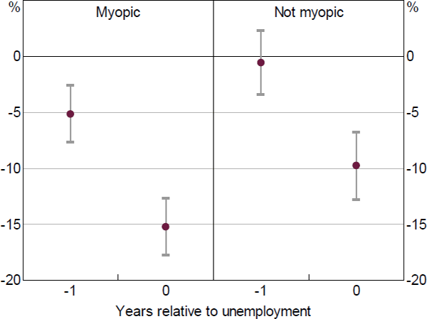
Note: Lines represent 95 per cent confidence intervals
Sources: Authors' calculations; HILDA Survey Release 19.0
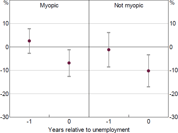
Note: Lines represent 95 per cent confidence intervals
Sources: Authors' calculations; HILDA Survey Release 19.0
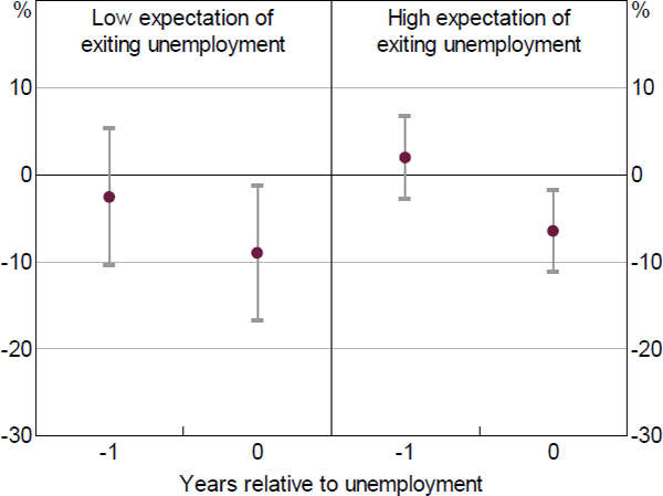
We also test whether, during unemployment, the consumption response varies by how long individuals expect to remain unemployed. To do this, we follow the same approach but split household heads into low (high) expectations of regaining work based on whether their expected probability of regaining work in the year ahead is below (above) 75 per cent (which is the mean response). We find larger consumption losses for unemployed workers that do not expect to regain employment within the year relative to those that do (Figures 16 and 17). This is consistent with these households smoothing consumption through a period of unemployment. However, these differences are not statistically significant.
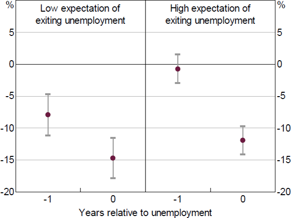
Note: Lines represent 95 per cent confidence intervals
Sources: Authors' calculations; HILDA Survey Release 19.0
Note: Lines represent 95 per cent confidence intervals
Sources: Authors' calculations; HILDA Survey Release 19.0
7. Sampling Bias in Household Surveys
A significant challenge in estimating the household spending response to unemployment using survey data is that unemployed survey respondents may not represent the ‘typical’ (or average) unemployment spell. In particular, the spell of unemployed survey respondents is generally longer than a typical spell (Salant 1977). This is because shorter spells are more likely to be ‘missed’ by the survey, as they occur in between waves. If the consumption response to unemployment varies with duration, then the estimates of consumption losses associated with unemployment may be biased and not representative of the typical unemployment experience.
This sampling bias is common to studies that try to identify the effect of unemployment on spending using survey data. To the best of our knowledge, there are few studies that attempt to address this issue, despite the fact that information on the length of unemployment is often available in longitudinal household surveys, such as the HILDA Survey.
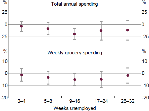
To explore the importance of this sampling bias, we test if the spending response to unemployment varies with how long the unemployed respondent has been reportedly searching for work. To do this, we re-estimate Equations (1) and (2) but include interaction effects for unemployment with ‘buckets’ of unemployment duration (e.g. 0–4 weeks, 5–8 weeks, etc).
We find that the consumption losses are larger for survey respondents that report being unemployed for longer spells at the time of the survey (Figure 18). Consumption losses are only statistically significant for those that have been unemployed for longer than a couple of months. This may imply that unemployment duration matters for a household's ability to smooth consumption over spells, or because workers who stay unemployed for longer are systemically different in ways that affect spending (such as wealth, household income, etc).
In summary, our estimates of consumption losses capture the effect of unemployment on the typical unemployed worker at a point in time. But our results may overstate the consumption losses associated with a typical unemployment spell given this is not the same concept. For instance, we do not capture the effect on respondents that are unemployed between survey waves, who are typically unemployed for shorter spells than the survey respondents that are observed to be unemployed. Having said this however, over-weighting the consumption falls of workers who remained unemployed for longer is appropriate for the purpose of capturing the aggregate effect of unemployment on aggregate spending.
Note: Lines represent 95 per cent confidence intervals
Sources: Authors' calculations; HILDA Survey Release 19.0
8. Conclusion and Policy Implications
We find that employed workers have some ability to predict whether they will lose their jobs in the year ahead. But they typically overestimate the probability of job loss. These systematic overestimations vary with the business cycle, with workers typically overestimating job loss during economic downturns and in the period just prior to the COVID-19 pandemic. Unemployed workers also underestimate the duration of the unemployment spell.
We find that household spending falls significantly at the onset of unemployment. Households also reduce spending by similar amounts regardless of whether the job loss is expected or not. However, households do cut back more on their spending if they expect a period of unemployment to persist. The effect of unemployment on spending is particularly strong for households that are liquidity constrained and during economic downturns. In contrast, we find only limited evidence that concerns about future job loss affect spending for those workers that do not become unemployed. Taken together, our results provide mixed evidence for the predictions of workhorse consumption models.
For policymakers, our research quantifies the effect of unemployment on spending, a previously unexplored aspect of unemployment in the Australian literature. Our findings highlight the cost of unemployment to households, and underscore the importance of macroeconomic policies that keep unemployment low. Our finding that households reduce spending by more the longer they remain unemployed may imply a role for policies designed to reduce unemployment duration.
Appendix A: Testing the Predictive Ability of Workers' Subjective Expectations
Here, we outline a simple model of expectations formation to more formally test the predictive ability of workers' subjective expectations. As well as testing whether subjective expectations contain predictive information for job loss above other observable variables, we examine whether worker expectations are fully rational, or whether their mistakes are systematic and predictable.
There is a significant body of literature in macroeconomics that tests the predictions of the workhorse model of expectations formation – the full information rational expectations (FIRE) hypothesis. There is also a large body of labour market research that studies the role of subjective expectations about employment. But there have been few studies that link these 2 lines of research. Most of the macro research has focused on surveys, typically of professional forecasters, and on how well they forecast aggregate variables like GDP growth and inflation. The studies on subjective expectations usually focus on the ability of individual workers to predict their own employment outcomes, but are less interested in what this tells us about how consumers form expectations and what this means for the macro economy. There are advantages to combining these 2 approaches using longitudinal data.
We adapt the framework of Keane and Runkle (1990) that tests the FIRE hypothesis based on a survey of professional forecasters. Expectations are assumed to be rational if they are equal to mathematical expectations conditional on the set of all information relevant to the worker. For an individual worker, we can express this relationship as:
Which states that the worker's expectation of employment next year is their (one-year-ahead) prediction of actual employment ( yit+1 ) based on the information set available to them at the time of the survey . This is equivalent to the statement expressed in terms of forecast errors:
For an individual worker the test of rationality involves running the regression:
where the dependent variable is the ‘true’ probability of job loss for worker i in survey year t + 1. In practice, the researcher does not observe the ‘true’ probability of job loss – we only observe the ex post binary outcome of whether a worker lost their job or not.
It is possible that beliefs about job prospects evolve differently across individuals over time. To allow for this, the equation also includes a set of control variables ( Xit ) for factors that may affect their willingness and ability to predict future job outcomes at a given point in time, such as the worker's age, sex, job tenure and industry of work.
The key explanatory variable is the worker's estimated probability of job loss in year t +1 as surveyed in year t. Under rational expectations, the estimated intercept should be zero , the slope coefficient on the subjective expectations should be equal to unity and the slope coefficients on the vector of control variables should be zero . Note that rational expectations allows individuals to hold different beliefs if they have different information sets (i.e. private information).
As Keane and Runkle (1990) argue, OLS estimates of the equation are likely to be biased. This is because the forecast errors across individuals could be correlated at a point in time (for example, because of an aggregate shock that affects job security in their industry). To partly address this, we specify the error term such that it includes both a worker fixed effect and an aggregate time fixed effect :
This simple adaption of the model provides a useful test of how worker expectations are formed. By including an individual worker fixed effect we allow for the possibility that an individual's forecast errors are correlated with an individual's time-fixed private information (e.g. previous forecast errors or their inherent ability). Because we have longitudinal information on individual workers and they are predicting their own outcomes, we can also test whether workers make systematic errors in aggregate. We do this by including time fixed effects. Many macro studies cannot follow this approach because the dependent variable is an aggregate variable being predicted by a range of forecasters at a specific point in time. The inclusion of time fixed effects would lead to perfect collinearity with the dependent variable, so the model could not be estimated.
We estimate the model above and test the FIRE hypothesis using 2 modelling approaches. The first approach is to estimate a linear probability (OLS) model for actual job loss on job loss expectations with (and without) individual worker fixed effects and controls. The second approach estimates a logistic regression because job loss is a binary outcome. The results of estimating Equation (A1) under the various approaches are shown in Table A1.
| OLS | OLS | Fixed effects | Logit | |
|---|---|---|---|---|
| Without controls | With controls | With controls | With controls | |
| Expected job loss | 0.18** (33.74) |
0.17*** (30.85) |
0.15*** (24.78) |
0.09*** (39.34) |
| Household fixed effects | No | No | Yes | No |
| Year fixed effects | No | Yes | Yes | Yes |
| R squared | 0.03 | 0.05 | 0.27 | 0.11 |
| Joint test (F-statistic) | F (1, 17,512) = 1,138.4 |
F (116, 17,378) = 19.7 |
F (115, 17,378) = 9.2 |
na |
| Observations | 114,822 | 111,806 | 111,806 | 111,806 |
|
Notes: ***, ** and * denote statistical significance at the 1, 5 and 10 per cent levels, respectively; standard errors are clustered by household, with t-statistics in parentheses; estimated coefficients on individual worker and year fixed effects not shown; regressions in columns 2 to 4 include control variables for demographics, such as age and education, and past labour force status, such as job tenure and the industry of work; see Appendix B for the full regression output; the joint test is a test that all the coefficients on the explanatory variables are jointly equal to zero Sources: Authors' calculations; HILDA Survey Release 19.0 |
||||
The results indicate that workers' subjective job loss expectations have some ability to predict actual job loss in the year ahead. Indeed, subjective expectations contain predictive power over and above the information observed by the econometrician about the worker. In each model specification, the regression coefficient on expected job loss is positive and significantly different from zero. A 1 percentage point increase in the expected probability of job loss is associated with an increase of about 10 to 18 basis points in the actual probability of job loss. This economic effect is small and t-tests confirm it is far from the value of one, pointing to a violation of rational expectations. These results are robust to changes in model specification, including the addition of lags on subjective expectations, and controlling for subjective response ‘bunching’ by including dummies for whether expectations are 0, 50 or 100 per cent. The inclusion of worker fixed effects causes the coefficient estimate for expected job loss to fall slightly (comparing columns 2 and 3 of Table A2). This points to a significant and correlated worker-specific component in both the true and expected probability of job loss.
We can also estimate the same model to test whether unemployed workers' expectations of job finding have predictive power for actual job finding rates. The results are shown in Table A2. Here, the sample is restricted to unemployed workers.
| OLS | OLS | Fixed effects | Logit(a) | |
|---|---|---|---|---|
| Without controls | With controls | With controls | With controls | |
| Expect to find employment within a year |
0.29*** (47.63) |
0.24*** (33.44) |
0.12*** (12.56) |
0.25*** (31.95) |
| Household fixed effects | No | No | Yes | No |
| Year fixed effects | No | Yes | Yes | Yes |
| R squared | 0.09 | 0.12 | 0.03 | 0.16 |
| Observations | 23,985 | 22,660 | 22,660 | 22,660 |
|
Notes: ***, ** and * denote statistical significance at the 1, 5 and 10 per cent levels, respectively; standard errors are clustered by household, with t-statistics in parentheses; estimated coefficients on year fixed effects not shown; regressions in columns 2 to 4 include control variables for demographics, such as sex, age and education; see Appendix B for the full regression output (a) Marginal effects Sources: Authors' calculations; HILDA Survey Release 19.0 |
||||
Again, expectations hold significant predictive power for future labour market outcomes. The subjective expectation of finding a job within the next 12 months is positively correlated with the actual rate of job finding over the period. This holds true even when we control for a range of worker characteristics, such as age and past labour force status. Notably, the inclusion of worker fixed effects causes the coefficient estimate to halve in size, which is again consistent with a fixed component to both expectations and realised unemployment duration, and indicates that individuals are good at predicting unemployment duration risk both overall and over time.
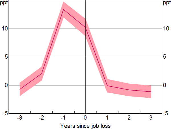
We can also exploit the longitudinal nature of the household-level data to examine how expectations of job loss evolve in the years just before and after a job loss event. To do this, we specify a model of job loss expectations with controls for time and individual fixed effects, and plot estimated coefficients on leads and lags of actual job loss. Using a fixed effects framework allows us to extract the component of job loss expectations that is correlated with a specific job loss event. We find that, for workers that lose their jobs, their subjective estimates of job loss rise in the 2 years leading up to the event (Figure A1).
This suggests that, despite evidence of bias, workers can predict actual labour market outcomes, even a few years out from the event. We also find that job loss expectations remain elevated in the year of the event, but one year later return to the same level as they were before the event.[21] This implies that there is no permanent change to individuals' job loss expectations following a job loss event.
Notes: Estimates are obtained from a linear fixed effects regression that includes year dummies; shaded area is 95 per cent confidence interval
Sources: Authors' calculations; HILDA Survey Release 19.0
Appendix B: Full Regression Output
Notes: Controls are added cumulatively; lines represent 95 per cent confidence intervals
Sources: Authors' calculations; HILDA Survey Release 19.0
| Dependent variable | Groceries | Meals eaten outside the home | Total expenditure |
|---|---|---|---|
| Unemployed | −0.05*** (0.01) |
−0.44*** (0.05) |
−0.06** (0.03) |
| Unemployed * lagged job loss probability | −0.04 (0.04) |
0.08 (0.15) |
−0.02 (0.07) |
| Lagged job loss probability | −0.01 (0.01) |
−0.06** (0.02) |
−0.04** (0.02) |
| Square root (number of household members) | 0.68*** (0.01) |
0.20*** (0.02) |
0.47*** (0.02) |
| Year (base = 2006) | |||
| 2007 | 0.10*** (0.01) |
0.07*** (0.03) |
0.04*** (0.01) |
| 2008 | 0.16*** (0.01) |
0.05* (0.03) |
0.10*** (0.01) |
| 2009 | 0.17*** (0.01) |
0.07** (0.03) |
0.07*** (0.01) |
| 2010 | 0.19*** (0.01) |
0.15*** (0.03) |
0.13*** (0.01) |
| 2011 | 0.24*** (0.01) |
0.25*** (0.03) |
|
| 2012 | 0.24*** (0.01) |
0.28*** (0.03) |
|
| 2013 | 0.25*** (0.01) |
0.27*** (0.03) |
|
| 2014 | 0.27*** (0.01) |
0.35*** (0.03) |
|
| 2015 | 0.28*** (0.01) |
0.38*** (0.03) |
|
| 2016 | 0.28*** (0.01) |
0.43*** (0.03) |
|
| 2017 | 0.28*** (0.01) |
0.40*** (0.03) |
|
| 2018 | 0.27*** (0.01) |
0.42*** (0.03) |
|
| 2019 | 0.30*** (0.01) |
0.47*** (0.03) |
|
| Constant | 3.80*** (0.01) |
3.75*** (0.04) |
9.63*** (0.03) |
| Fixed effects | Yes | Yes | Yes |
| R squared (overall) | 0.20 | 0.02 | 0.07 |
| Observations | 96,060 | 91,461 | 30,558 |
|
Notes: ***, ** and * denote statistical significance at the 1, 5 and 10 per cent levels, respectively; p-values are in parentheses Sources: Authors' calculations; HILDA Survey Release 19.0 |
|||
References
Aguiar M and E Hurst (2005), ‘Consumption versus Expenditure’, Journal of Political Economy, 113(5), pp 919–945.
Attneave F (1953), ‘Psychological Probability as a Function of Experienced Frequency’, Journal of Experimental Psychology, 46(2), pp 81–86.
Been J, E Suari-Andreu, M Knoef and R Alessie (2020), ‘Consumption Responses to Unemployment’, Network for Studies on Pensions, Aging and Retirement Academic Series, Netspar Discussion Paper DP 01/2020-005.
Browning M and TF Crossley (2001), ‘Unemployment Insurance Benefit Levels and Consumption Changes’, Journal of Public Economics, 80(1), pp 1–23.
Burbidge JB, L Magee and AL Robb (1988), ‘Alternative Transformations to Handle Extreme Values of the Dependent Variable’, Journal of the American Statistical Association, 83(401), pp 123–127.
Chetty R and A Szeidl (2007), ‘Consumption Commitments and Risk Preferences’, The Quarterly Journal of Economics, 122(2), pp 831–877.
Christelis D, D Georgarakos and T Jappelli (2015), ‘Wealth Shocks, Unemployment Shocks and Consumption in the Wake of the Great Recession’, Journal of Monetary Economics, 72, pp 21–41.
Cullen JB and J Gruber (2000), ‘Does Unemployment Insurance Crowd out Spousal Labor Supply?’, Journal of Labor Economics, 18(3), pp 546–572.
Dickerson A and F Green (2012), ‘Fears and Realisations of Employment Insecurity’, Labour Economics, 19(2), pp 198–210.
Foster J and R Guttmann (2018), ‘Job Security Perceptions and Its Effects on Wage Growth’, Australian Journal of Labour Economics, 21(3), pp 229–251.
Ganong P and P Noel (2019), ‘Consumer Spending during Unemployment: Positive and Normative Implications’, The American Economic Review, 109(7), pp 2383–2424.
Gruber J (1997), ‘The Consumption Smoothing Benefits of Unemployment Insurance’, The American Economic Review, 87(1), pp 192–205.
Hendren N (2017), ‘Knowledge of Future Job Loss and Implications for Unemployment Insurance’, The American Economic Review, 107(7), pp 1778–1823.
Jappelli T and L Pistaferri (2017), The Economics of Consumption, Theory and Evidence, Oxford University Press, New York.
Kaplan G, GL Violante and J Weidner (2014), ‘The Wealthy Hand-to-Mouth’, Brookings Papers on Economic Activity, Spring, pp 77–138.
Keane MP and DE Runkle (1990), ‘Testing the Rationality of Price Forecasts: New Evidence from Panel Data’, The American Economic Review, 80(4), pp 714–735.
Khaw MW, L Stevens and M Woodford (2021), ‘Individual Differences in the Perception of Probability’, PLOS Computational Biology, 17(4), e1008871.
Kleinjans KJ and A van Stoest (2010), ‘Nonresponse and Focal Point Answers to Subjective Probability Questions’, Institute for the Study of Labor, IZA Discussion Paper No 5272.
Krolikowski P (2017), ‘Measuring the True Impact of Job Loss on Future Earnings’, Federal Reserve Bank of Cleveland Economic Commentary No 2017-11.
Lancaster D (forthcoming), ‘The Financial Cost of Job Loss in Australia’, RBA Bulletin.
Landais C and J Spinnewijn (2019), ‘The Value of Unemployment Insurance’, Centre for Economic Policy Research Discussion Paper DP13624, rev 25 June 2019.
Malmendier U and LS Shen (2021), ‘Scarred Consumption’, Unpublished manuscript, 17 January. Available at <https://static1.squarespace.com/static/5bbd7f9165019f8db3ff3f07/t/600df2f79cedb068d2ce1ab5/1611526903955/Draft_MalmendierShen_12jan2021.pdf>.
Manski CF and JD Straub (2000), ‘Worker Perceptions of Job Insecurity in the Mid-1990s: Evidence from the Survey of Economic Expectations’, The Journal of Human Resources, 35(3), pp 447–479.
McGuinness S, M Wooden and M Hahn (2014), ‘The Perceived Probability of Job Loss and Future Labour Market Outcomes’, Industrial Relations Journal, 45(4), pp 329–347.
Meyer BD and JX Sullivan (2003), ‘Measuring the Well-Being of the Poor Using Income and Consumption’, The Journal of Human Resources, 38(Special Issue on Income Volatility and Implications for Food Assistance Programs), pp 1180–1220.
Mueller AI, J Spinnewijn and G Topa (2021), ‘Job Seekers’ Perceptions and Employment Prospects: Heterogeneity, Duration Dependence, and Bias', The American Economic Review, 111(1), pp 324–363.
Salant SW (1977), ‘Search Theory and Duration Data: A Theory of Sorts’, The Quarterly Journal of Economics, 91(1), pp 39–57.
Spinnewijn J (2015), ‘Unemployed but Optimistic: Optimal Insurance Design with Biased Beliefs’, Journal of the European Economic Association, 13(1), pp 130–167.
Stephens M, Jr (2004), ‘Job Loss Expectations, Realizations, and Household Consumption Behavior’, The Review of Economics and Statistics, 86(1), pp 253–269.
Varey CA, BA Mellers and MH Birnbaum (1990), ‘Judgments of Proportions’, Journal of Experimental Psychology: Human Perception and Performance, 16(3), pp 613–625.
Wilkins R and C Sun (2010), ‘Assessing the Quality of the Expenditure Data Collected in the Self-Completion Questionnaire’, Melbourne Institute of Applied Economic and Social Research, HILDA Project Discussion Paper Series No 1/10.
Acknowledgements
We would like to thank Benjamin Beckers, James Bishop, Iris Chan, Adam Gorajek, James Hansen, Calvin He, Amanda Martz, John Simon and seminar participants at the Reserve Bank of Australia. The views expressed in this paper are those of the authors and do not necessarily reflect the views of the Reserve Bank of Australia. The authors are solely responsible for any errors.
Footnotes
Gruber (1997), Browning and Crossley (2001), Chetty and Szeidl (2007), Christelis, Georgarakos and Jappelli (2015) and Hendren (2017) calculate consumption losses from unemployment in the United States, and Landais and Spinnewijn (2019) does the same for Sweden. [1]
Technically, the ‘food’ spending measure includes food, meals eaten out and other grocery spending (which includes cleaning and personal care products). [2]
Previous research has found that there can be large discrepancies amongst survey respondents within the same household in terms of reporting total spending in the HILDA Survey (Wilkins and Sun 2010). Grocery expenditure has been found to be the most consistent estimate within households. [3]
This finding is also apparent in the US data (Mueller et al 2021). [4]
If conservatism fully explains the cross-sectional pattern in job loss expectations we might expect ‘mean reversion’, in which the difference between the expected and model-based estimates decreases with the level of actual job loss. Partly arguing against this interpretation, we find that the deviation between the subjective and model-based estimates of job loss increases in both the level of actual job loss and the level of expected job loss. [5]
See Meyer and Sullivan (2003) for further discussion of economic measures of wellbeing. [6]
Gruber (1997), Browning and Crossley (2001), Chetty and Szeidl (2007) and Christelis et al (2015) estimate consumption losses from unemployment in the United States, and Landais and Spinnewijn (2019) does the same for Sweden. [7]
See Salant (1977) for more information on length-biased sampling and the implications for unemployment data. [8]
The household ‘head’ is identified in the HILDA Survey by applying the following criteria, in order, until a unique person is selected. The criteria are: i) a registered or de facto marriage; ii) a long parent; iii) the person with the highest financial year income; and iv) the eldest person. We use the household head status in the previous year as the head selection criteria. [9]
See Krolikowski (2017) for a discussion of the problems associated with estimating causal effects of unemployment. [10]
If other household members increase their hours in response to unemployment of the head, these estimates may be understated. However, the literature finds little empirical support for this (Cullen and Gruber 2000). It is also likely that consumption effects are larger for single-income families than those presented here. [11]
Specifically, the controls are the age and education level of the household head, contract type (e.g. permanent, casual or fixed term) and industry of work. We also re-estimate all specifications in first differences and find no substantive differences in our results. [12]
The survey respondents are asked to report spending in ‘a normal week’, which could be interpreted as the period before unemployment. As a result, while the results are similar to the literature, it is possible that the estimates are understated. [13]
We use the inverse hyperbolic sine of weekly wages of the entire household. [14]
When income returns to levels comparable with households that had never experienced unemployment, the dashed lines and solid lines meet in Figures 10 through 12, indicating income plays no explanatory role. [15]
While we only consider wage income in these specifications, the fall in total income (including public transfers) would explain even less of the observed fall in expenditure at unemployment. This is because public transfers rise during unemployment. [16]
We find other sources of heterogeneity in the spending response to job loss, including personal characteristics such as age and income. The effect of job loss on spending varies with age. Specifically, it appears to be a quadratic function of age, with households where the head is aged 45 to 54 most sensitive to unemployment. Two factors may drive this relationship. First, younger households have more time over which to smooth the earnings losses from unemployment. Thus the PIH would imply that they respond less to earnings losses. Second, older households are less likely to be liquidity constrained, and as a result more able to smooth the effect of unemployment. The effect of job loss on spending also varies with the level of household income. Low-income households experience the largest reductions in spending. This is consistent with low-income households being more liquidity constrained. However, even high-income households reduce spending in response to job loss. [17]
We also tested whether job loss expectations affect spending in the modelling framework of Stephens (2004). We found similar results in that there is no evidence that anticipated job losses affect spending. We also tested all the spending regressions with a Poisson fixed effects model instead of a log linear model and the results were unchanged. [18]
As the hand-to-mouth variable is constructed using variables only available in the wealth module, and total expenditure is only available for a small subset of the sample, we are unable to estimate the total expenditure response to unemployment by hand-to-mouth status. [19]
Under the Kaplan et al (2014) framework, households are considered ‘hand-to-mouth’ if their fortnightly income is greater than or equal to their current liquid net wealth. [20]
We are able to elicit job loss probabilities from respondents in the year of job loss (year t ) since the majority of those who lost their job go on to regain employment before the time of the survey. [21]