RDP 2021-07: Macroprudential Limits on Mortgage Products: The Australian Experience 7. Other Mortgage Market Outcomes
July 2021
- Download the Paper 2,356KB
This section analyses policy effects on other outcomes of interest, and the cyclicality of mortgage commitments throughout the sample. The first part shows how APRA's soft guidance on LVRs interacted with the mortgage growth limits. The second part looks at how the policies affected aggregate variables related to total credit growth, banking market share and banks' mortgage interest income. The third part discusses an unintended side effect of the investor policy – customers switching the classification of their loan from investor to occupier. The fourth part discusses some results for mortgage commitments behaviour throughout the sample.
7.1 Policy effects by loan-to-valuation ratio
The two macroprudential limits were accompanied by guidance from APRA that banks should manage their high-LVR lending. When announcing the investor policy, LVRs were only mentioned briefly. APRA stated that it would generally lift scrutiny over higher risk lending, and gave several examples of higher risk lending that included ‘lending at high loan-to-valuation ratios’ (APRA 2014). When announcing the IO policy, the advice was more explicit. Banks were asked to:
… place strict internal limits on the volume of interest-only lending at loan-to-valuation ratios (LVRs) above 80 per cent; and
… ensure there is strong scrutiny and justification of any instances of interest-only lending at an LVR above 90 per cent … (APRA 2017).
This subsection separates mortgage commitments into 3 LVR buckets and analyses the policy effects separately for each. This serves 2 purposes. First, it tests whether the results in Sections 5 and 6 could simply be picking up APRA's guidance on LVRs, given that targeted loan types can have higher LVRs. If this was the case, then regressions that hold LVRs constant would show the same policy effects in targeted and non-targeted loan types. Second, it provides additional understanding of how the overall policy packages affected mortgages of different LVRs.
The analysis is approached with some modifications to the commitments growth regressions in Sections 5 and 6. To distinguish commitments by LVR, we add an LVR dimension ( l ) to the dataset. This basically means creating 3 datasets for different LVR buckets – LVR ≤ 80%; 80% < LVR ≤ 90%; and LVR > 90% – and stacking them together to form a bank-quarter-LVR-level dataset. The policy effects are then estimated separately for each LVR bucket, by interacting the policy indicator variable with an indicator variable for the LVR level. To capture the results in a concise set of coefficients, the 4 policy indicator lags used in the previous regressions are replaced with a single policy indicator that equals one in both of the 2 quarters in which the policies had most effect, as informed by the previous results (i.e. for the investor policy, 2015:Q3 and Q4, and for the IO policy, 2017:Q2 and Q3). Instead of using first differences and the Arrellano-Bond instrumental variables method, the regressions include fixed effects at the bank × LVR bucket level. Data are not available for IO commitments, so for both policies, we compare investor and occupier commitments, which means the results for IO policy effects are less reliable.
Specifically, the regression equations are
The results show that the policy effects found in Sections 5 and 6 are not simply capturing LVR effects (Table 8). Within each LVR bucket, the policy effect coefficients are consistently more negative for investor commitments than for occupier commitments. In particular, the effect of investor limit on investor commitments is strongest in the highest LVR bucket, while in that bucket there is virtually no policy effect on occupier commitments.
| Sample banks: |
(a) | (b) | (c) | (d) | |
|---|---|---|---|---|---|
| Large | Mid-sized | ||||
| Commitments type: | Investor | Occupier | Investor | Occupier | |
| Investor policy regressions | |||||
| 𝕀(LVR ≤ 80)×𝕀(Invpolicy) | −0.189 (0.122) |
0.154* (0.091) |
−0.263** (0.116) |
0.016 (0.081) |
|
| 𝕀(80 < LVR ≤ 90)×𝕀(Invpolicy) | −0.095 (0.122) |
0.199** (0.091) |
−0.298** (0.120) |
−0.067 (0.082) |
|
| 𝕀(LVR > 90)×𝕀(Invpolicy) | −0.511*** (0.123) |
0.004 (0.091) |
−0.405*** (0.128) |
−0.019 (0.081) |
|
| R squared | 0.116 | 0.084 | 0.094 | 0.066 | |
| Sample | 528 | 528 | 1,811 | 1,996 | |
| IO policy regressions | |||||
| 𝕀(LVR ≤ 80)×𝕀(IOpolicy) | −0.033 (0.124) |
0.032 (0.091) |
−0.094 (0.103) |
−0.016 (0.071) |
|
| 𝕀(80 < LVR ≤ 90) × 𝕀(IO policy) | −0.107 (0.124) |
0.044 (0.091) |
−0.198* (0.107) |
−0.067 (0.071) |
|
| 𝕀(LVR > 90)×𝕀(IOpolicy) | −0.192 (0.124) |
−0.022 (0.091) |
−0.300** (0.123) |
−0.193*** (0.072) |
|
| R squared | 0.087 | 0.072 | 0.088 | 0.069 | |
| Sample | 528 | 528 | 1,811 | 1,996 | |
| Fixed effects | Bank × LVR | Bank × LVR | Bank × LVR | Bank × LVR | |
| Other controls | yes | yes | yes | yes | |
| Notes: Coefficients from regressions at the bank–quarter–LVR bucket level, as specified in Equation (4). The controls include 2 lagged dependent variables, to be consistent with the regressions in Sections 5 and 6. The lagged dependent variables deal with any autocorrelation, in the same manner as in the Section 5 and 6 regressions, so the standard errors are not additionally clustered. ***, ** and * denote statistical significance at the 1, 5 and 10 per cent levels, respectively. | |||||
Notwithstanding this, the policies do have a significant effect on the LVR distribution, in line with APRA's guidance. Declines in targeted mortgages are concentrated in the highest LVR bucket, and rises in non-targeted mortgages are concentrated in lower LVR buckets. Mid-sized banks reduce low-LVR credit in targeted mortgages more so than large banks, but the strongest effect for mid-sized banks is still clearly in the highest LVR loans. APRA's guidance on LVRs appears to have interacted with the mortgage limits by determining, within each type of mortgage, at what LVRs the reactions occur.
7.2 Policy effects on aggregate variables
This section analyses policy effects on aggregate variables of interest. The analysis uses time series regressions that regress the outcome variable on various controls, including lagged dependent variables. The exact specifications are discussed in each subsection, and resemble Equations (1) and (2) with the cross-section collapsed into a single series. The time series samples are small, so we report these results in placebo regression figures as in Sections 5.4.1 and 6.4. These sets of estimates nest the estimated policy effects, which are the ‘placebo’ coefficients for the quarters when the policies were actually implemented. Comparing the full set of ‘trend deviation’ coefficients also indicates the reliability of the estimated policy effects, in the same manner as the placebo regressions presented earlier. To reiterate, the results show a statistically significant policy effect if, during the policy quarters, the coefficient's 95 per cent confidence interval is fully above or below zero. The fewer significant effects outside the policy period, the more robust any estimated policy effects are.
7.2.1 Effects on aggregate housing and business credit growth
The results in Sections 5 and 6 analyse bank-level credit reactions, but do not measure the policy effect on total housing credit, because those regressions weight each of the sample banks equally. To formally test for effects on credit aggregates we estimate
The dependent variable CreditGrth takes on 4 definitions: total investor housing credit, total occupier housing credit, total (domestic) housing credit and total (domestic) business credit.[23] (Reliable aggregates for IO and P&I housing credit are not available.) As discussed above, this regression is repeated multiple times while rolling the quarter in 𝕀(quarter)t across all quarters from 2010 to 2019. The vector Controlst includes GDP growth, housing price growth, the first difference of the cash rate and its first lag, the average capital ratio across sample banks, the average deposit ratio across sample banks, and a set of seasonal indicators. These variables are defined as in Section 3.2.
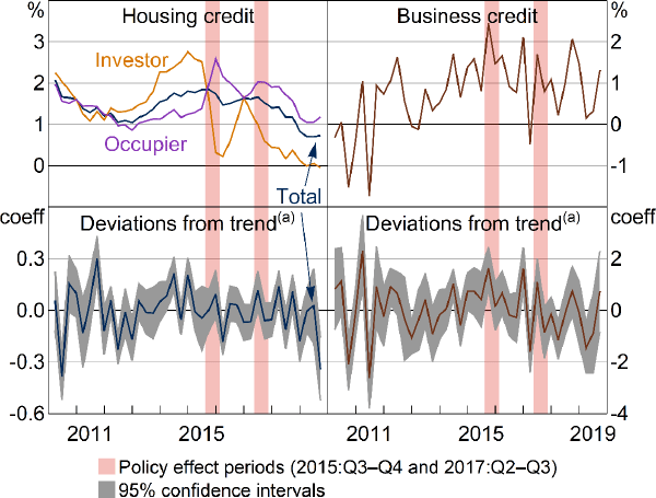
The raw data and the regression results both suggest that the policies had little effect on banks' total housing credit (Figure 10, left panels). While each policy coincided with a decline in investor credit growth and a pick-up in occupier credit growth, total housing credit growth remained relatively flat. (Aggregate credit growth data are not available for IO mortgages, but, as evident in Figure 1, the IO share of investor loans is higher than that of occupier loans.) Credit growth dropped just after the investor policy period, but this was driven by a decline in occupier growth. APRA (2019b) also concludes that, for the investor policy, the aggregate trend in housing credit growth remained broadly unchanged.

Note: (a) Coefficient estimates from rolling ‘placebo’ regressions, described in text
Sources: Authors' calculations; RBA Statistical table D1 Growth in Selected Financial Aggregates
Next, CreditGrtht is defined as banks' total domestic business credit growth. The policies could feasibly affect business credit for at least 2 reasons. Banks might substitute away from the targeted mortgage type and into business credit, similar to the effect for large banks in occupier credit during the first policy. This would cause a pick-up in business credit. Alternatively, business credit could be neglected as banks concentrate more resources on controlling their mortgage portfolio. This would cause a decline in business credit.
There is evidence for a pick-up in business credit growth during the investor policy (Figure 10, bottom right panel). The trend deviation is larger and has a higher significance level than any trend deviation coefficients since 2011. This result is consistent with a substitution into business credit by banks compensating for less investor mortgage origination. There is no significant effect for the IO policy.
7.2.2 Effects on market concentration
Sections 5 and 6 show that large banks substitute into non-targeted mortgage types while mid-sized banks do not. This section tests whether the different responses resulted in the large banks increasing their mortgage market share relative to the mid-sized banks. We conclude that large banks' IO policy-induced substitution into P&I loans likely had a positive single-quarter effect on their mortgage market share relative to the 20 or so mid-sized banks in our sample, and this was at the expense of large banks' mortgage interest income.
The analysis re-estimates Equation (5), but replaces CreditGrtht with 1 of 2 measures of large banks' market share: their mortgage interest income (MII) as a proportion of the total across sample banks; and their quarterly dollar change in mortgage credit outstanding as a proportion of the total across sample banks.[24] For the MII regressions, the cash rate control variables are included as levels rather than first differences, because mortgage interest rates are closely related to the cash rate level. Both dependent variables are sourced from the APRA dataset noted in Section 3.1.
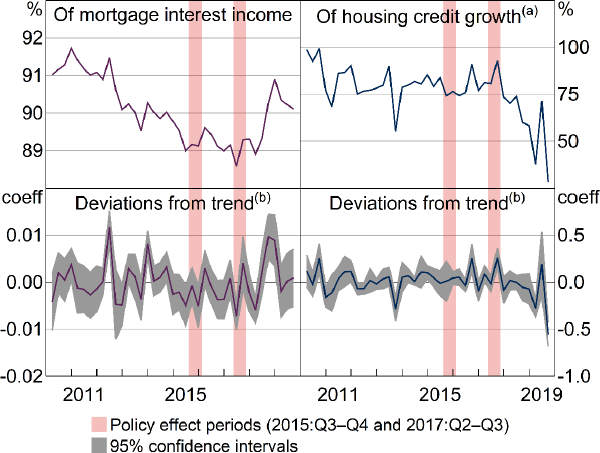
Large banks' MII share significantly drops during the IO policy period, in 2017:Q2 Figure 11, bottom left panel). This is likely driven by their bigger decline in IO commitments growth relative to midsized banks (Section 6.1), which reflects their higher share of IO commitments prior to the policy. The effect appears temporary: large banks' MII share is above trend in 2017:Q3, but not significantly (bottom left panel), and the rebound is visible in the raw data (top left panel).

Notes:
(a) Large banks' quarterly change in credit (in $) divided by all banks' quarterly change in credit
(b) Coefficient estimates from rolling ‘placebo’ regressions, described in text
Sources: APRA; Authors' calculations; RBA
Large banks' share of credit growth across sample banks significantly rises in 2017:Q3 before dropping again (Figure 11, bottom right panel). The timing matches their substitution into P&I commitments growth (Table 5), and may be the driver of their rebound in MII share. The effect again appears temporary: their share of credit growth drops and is below trend in all of the following few quarters (right panels).
The investor policy has no statistically significant effect on large banks' share of MII or of mortgage credit growth (Figure 11, bottom panels). The raw data show that large banks' share of MII picks up after the investor policy (top left panel), but the regression results show that it is not a statistically significant deviation from trend (bottom left panel), and therefore likely unrelated to the policy.
7.2.3 Effects on banks' pricing power
The Australian Government Productivity Commission (PC) has criticised the policies for their competition implications. PC (2018, p 180) writes:
Under the benchmark interventions, any ADI charging a materially lower interest rate than its competitors would receive an outsized number of loan applications that, if approved, could result in it breaching APRA's growth limit for the investor segment. As a result, ADIs increased their pricing for investor and interest-only lending — including both new and existing loans — or temporarily discontinued cheaper products …
Notwithstanding this, PC (2018) also concludes that swift action by APRA was appropriate and that APRA's proposed risk weight changes are an appropriate tool going forward. The ACCC has reached similar conclusions to the PC. ACCC (2018a, p 42) writes:
While APRA's interest-only benchmark had the objective of contributing to financial system stability, we find it lessened price competition for interest-only lending. We consider that the benchmark provided the opportunity for the banks to synchronise their significant increases to interest-only rates during the price monitoring period, at a significant cost to those borrowers.
Ultimately, the PC and ACCC concerns are that the policies lifted banks' ability to extract surplus value from customers (in a microeconomic sense), by inducing a softening of pricing competition between banks. To analyse this, we look at reactions in banks' total MII. A change in prices alone does not reveal competition effects, because the price change could be exogenously driven – for example, by new information about loan riskiness or potential future funding costs – and customers' demand reductions could still be consistent with a competitive market, with substitution into competing products. The main difference between a competitive and a monopolistic market is in the price elasticity of demand (e.g. Dixit and Stiglitz 1977). The implication is that, if a price rise is driven by a lift in monopolistic power, income should also pick up, with the monopolist benefiting from the combination of the price rise and customers' demand insensitivity.
To test whether the policies caused a pick-up in MII, we re-estimate Equation (5) but replace CreditGrtht with the cross-sectional sum of sample banks' housing interest income (from the same APRA dataset). As in the MII analysis in Section 7.2.2, the cash rate control variables are included as levels rather than first differences.[25]
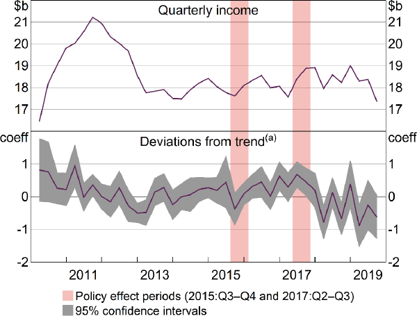
MII is significantly above trend in both of the IO policy quarters (Figure 12, bottom panel). There is also a positive significant trend deviation in 2016:Q4, which could have been a delayed reaction to the investor policy, but this is less conclusive and is not apparent in the raw data (top panel). Either way, the significant deviations in the IO policy period are consistent with the hypothesis that the IO policy temporarily lifted banks' monopolistic pricing power. Combining this result with the results in Section 7.2.2 suggests that the monopolistic benefit went to mid-sized banks initially (in 2017:Q1), before spreading across all banks (in 2017:Q2). It is worth noting, however, that competition and financial stability can conflict with each other. For example, APRA's letter to ADIs about the investor policy notes that strong competition in the housing market was pushing lending standards down (APRA 2014). The potential conflict is also well established in the empirical and theoretical banking literature (e.g. Freixas and Rochet 2008; Berger, Klapper and Turk-Ariss 2017).

Note: (a) Coefficient estimates from rolling ‘placebo’ regressions, described in text
Sources: APRA; Authors' calculations
7.3 Loan-type switching
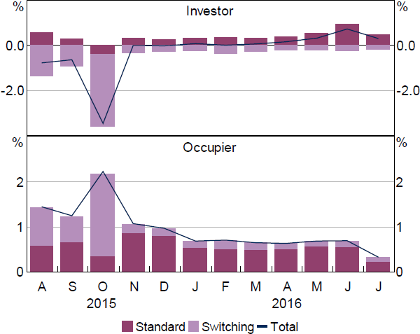
When the investor policy was implemented, regulators observed that many existing borrowers were reclassifying themselves from investor to occupier. That is, borrowers who were investors at origination were notifying their bank that they were now occupiers. The policy caused incentives for borrowers to do this, to receive a lower interest rate (Section 5.2). Banks may have also initially thought that this loan-type switching would help them to meet the investor credit growth limit, although APRA has noted that it measured credit growth by looking through loan-type switching (APRA 2019b). APRA began asking banks for monthly data on loan-type switching in July 2015 (Figure 13). From July to October 2015, credit growth from loan-type switching dominated standard credit growth.

Source: RBA
This policy-induced loan-type switching is one of the reasons we use mortgage commitments as the dependent variable for our credit quantity regressions. Commitments should be less affected than credit growth by loan-type switching, because customers typically do not have to make a new loan application to switch their loan type within the same bank. However, commitments may not completely remove loan-type switching effects, because some customers could go to the extra effort of switching by applying for refinancing at a new bank, potentially to take advantage of lower rates at that bank. To the extent that this occurred, our investor policy effects may be overestimated.
7.4 The cyclicality of mortgage products
The commitments regressions in Sections 5.1 and 6.1 include macroeconomic control variables whose coefficients are informative about the general behaviour of commitments growth. However, those regressions group mortgage types together within the targeted and non-targeted categories, which is appropriate for analysing policy effects, but less so for analysing general mortgage behaviour. Here we report control coefficient estimates that are more definitive by running separate regressions on the 4 mortgage subtypes: occupier P&I, occupier IO, investor P&I and investor IO. These regressions re-estimate Equation (1) (with different definitions of m ), but include all 8 policy indicators in each regression (4 each for the investor and IO policies).
Housing prices correlate with investor commitments and IO commitments, but not with occupier P&I commitments (Table 9). This may suggest that speculative demand for housing is in part driven by extrapolation of recently observed house prices (e.g. extrapolative expectations are discussed in Armona, Fuster and Zafar (2019)), in line with prevailing views on the Australian housing market (e.g. APRA 2019b). This effect is stronger for large banks than for mid-sized banks; we do not speculate on why. Basten and Koch (2015) find a positive causal relationship of housing prices on mortgage demand. Our findings build on their results by showing that this holds true only for housing investors, at least in Australia. The lack of relationship with occupier P&I credit, which in Australia is the largest housing credit category (Figure 1), is consistent with the cross-country panel findings in Kearns, Major and Norman (2020) that, in aggregate, housing prices do not have a positive effect on household debt.
| Dependent variable: |
(a) | (b) | (c) | (d) | (e) | (f) | (g) | (h) | |||
|---|---|---|---|---|---|---|---|---|---|---|---|
| Occupier P&I | Investor P&I | Occupier IO | Investor IO | ||||||||
| Sample banks: | Large | Mid-sized | Large | Mid-sized | Large | Mid-sized | Large | Mid-sized | |||
| GDP | 0.055 (0.043) |
0.101*** (0.034) |
0.042* (0.025) |
0.111* (0.064) |
−0.005 (0.051) |
0.004 (0.070) |
−0.028 (0.039) |
0.055 (0.043) |
|||
| Housing prices | 0.003 (0.007) |
−0.001 (0.008) |
0.036*** (0.009) |
0.003 (0.011) |
0.015*** (0.004) |
0.017* (0.010) |
0.018* (0.011) |
0.003 (0.007) |
|||
| Lagged DVs | 2 | 2 | 2 | 2 | 2 | 2 | 2 | 2 | |||
| Policy indicators | 8 | 8 | 8 | 8 | 8 | 8 | 8 | 8 | |||
| Other controls | yes | yes | yes | yes | yes | yes | yes | Yes | |||
| Sample | 168 | 624 | 168 | 621 | 168 | 620 | 168 | 168 | |||
| Notes: Coefficients from panel regressions, across banks and quarters, of granular categories of commitments growth on quarterly GDP growth and quarterly housing price growth. The full equation is in first differences, using Arellano–Bond, with 2 lagged dependent variables (to eliminate second order autocorrelation). Other controls include all 8 policy indicator variables, seasonal indicators and the bank-level control variables (capital and deposits). For the mid-sized banks' regression of occupier IO commitments, only 2 seasonal indicators are used, to avoid multicollinearity with instruments. ***, ** and * denote statistical significance at the 1, 5 and 10 per cent levels, respectively. | |||||||||||
GDP correlates with P&I commitments but not IO commitments (Table 9), and the effect is stronger for mid-sized banks than for large banks. Income is an intuitive driver of general mortgage commitments through its link with borrowing capacity. A plausible explanation for its lack of relationship with IO commitments is that IO commitments have their own structural drivers. For example, between 2011 and 2014, when aggregate IO lending was growing strongly and housing price growth was picking up, GDP growth was trending downwards (Figure 1). This structural shift in IO lending is also noted in ASIC (2015).
Footnotes
The CreditGrtht variables are of Australian credit aggregates, taken from RBA Statistical table D1 (available at <https://www.rba.gov.au/statistics/tables/>). These data have broader coverage than the bank-level samples in previous sections. For housing credit, contributions of non-sample banks would be minimal. For business credit, contributions of non-sample banks – namely foreign bank branches – is likely more noticeable. As these banks should be much less affected by the policies, their inclusion may be biasing the estimated policy effects on business credit towards zero. [23]
Changes in mortgage credit outstanding are strictly positive for both large and mid-sized groups throughout the sample. [24]
One large bank has an immense trough then spike in 2016:Q1 and Q2 that dominates the aggregate MII movements. We assume it does not reflect true income changes, and replace these 2 values with their mean across those 2 quarters. This adjustment lifts the aggregate 2016:Q1 outcome by $1.03 billion and lowers the aggregate 2016:Q2 outcome by $1.03 billion. [25]