RDP 2019-01: A Model of the Australian Housing Market 4. Main Equations
March 2019
4.1 Building Approvals
We model constant price building approvals for detached houses, higher-density housing, and alterations and additions separately.[1] This disaggregation is useful because the different types of construction behave differently and because alterations and additions do not contribute to the number of new dwellings, an important factor in explaining the vacancy rate. In Section 4.2 we then discuss how these equations are mapped into dwelling investment and completions. Modelling approvals – rather than dwelling investment as many other researchers do – has a couple of advantages. Approvals lead dwelling investment so should improve near-term forecasts. The earlier timing reduces scope for explanatory variables to react, allaying endogeneity concerns. It reduces the lag from shocks to observed decisions. And it facilitates distinctions between the number and value of new dwellings, a feature we exploit in modelling vacancies in Section 4.3.
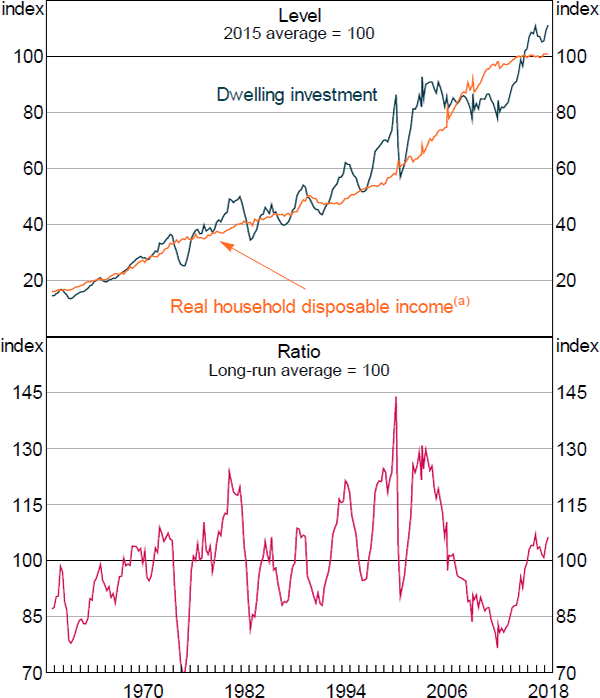
There are several key features of the data that the model needs to reflect. First, as shown in Figure 2, dwelling investment has grown at a similar rate to real income over the past 60 years, with the ratio between these variables fluctuating around a fairly stable mean. Approvals data show a similar nexus but are only available from 1973. It might seem unsurprising that construction activity grows in line with the rest of the economy, however this is not a feature of some other models, for example Ball, Meen and Nygaard (2010, Table 2).
As we note below, the stability of the ratio in Figure 2 (bottom panel) means that other highly persistent variables, such as real interest rates, real construction costs or real housing prices, do not have large long-run effects on investment, even though some theories suggest they should. Accelerator models suggest that the level of net investment should depend on the growth, as well as the level, of income. However, we do not find the growth in income to have explanatory power. As can be seen in Figure 2 (top panel), the rapid mining-driven growth in income in the 2000s was accompanied by sluggish dwelling investment (from a high starting point). Slow growth in income over the past decade was accompanied by a construction boom.
Note: (a) Before interest payments, including unincorporated enterprises; deflated by trimmed mean CPI from 1982 onwards and headline CPI prior to this
Sources: ABS; RBA
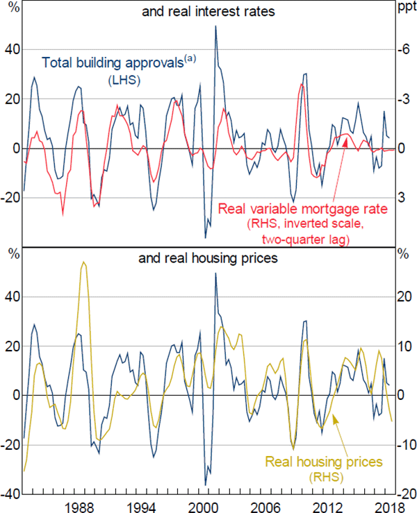
Second, in the short run, construction activity seems to be highly responsive to changes in interest rates (Figure 3, top panel) and changes in existing housing prices (bottom panel).
Notes:
All series are year-ended changes
(a) Alterations and additions have been scaled to be representative of their share of national accounts dwelling investment
Sources: ABS; Corelogic; RBA
Reflecting these stylised facts, our three equations for building approvals each take the following form:
where app is a constant price measure of building approvals, hhdy is real household disposable income, R is the real discounted mortgage rate, dp is the real dwelling price, GST is a dummy variable equal to one in the September quarter 2000 and zero otherwise, and ϕ is a time-varying intercept. Lower case variables are in natural logs. All variables in log differences have been demeaned. We estimate from March quarter 1987, following the deregulation of mortgage interest rates, to June quarter 2018. It was common to model dwelling investment before this period as credit constrained (see Jovanoski et al (1997, pp 11–12); Williams (1984)). A summary of estimates is in Table 1. More detailed estimates are provided in tables E1, E2 and E3 of Online Appendix E.
| Regressor | Detached houses | Higher-density housing | Alterations and additions |
|---|---|---|---|
| −0.10** (0.048) |
−0.21 (0.14) |
−0.18* (0.097) |
|
| 0.19** (0.092) |
−0.60*** (0.19) |
−0.24*** (0.092) |
|
| −0.062*** (0.014) |
−0.11*** (0.043) |
−0.037** (0.016) |
|
| 0.70** (0.33) |
3.0*** (0.95) |
0.77** (0.33) |
|
| −0.50** (0.21) |
−0.49 (0.79) |
−0.39 (0.31) |
|
| Notes: ***, ** and * denote significantly different from zero at 1, 5 and 10 per cent levels, respectively; standard errors are in parentheses | |||
We interpret the causation in our equations as running from right-hand side variables to the left-hand side. As noted earlier, we do not prove this, but it strikes us as a natural interpretation. Assumptions of reverse causation – for example, that residuals in the approvals equations cause earlier changes in interest rates – are inconsistent with our understanding of the monetary policy process and the information available to the central bank. Moreover, reverse causation would give rise to a positive correlation, biasing our coefficients towards zero and strengthening our results.
Subject to that qualification, several features of the estimates are worth noting:
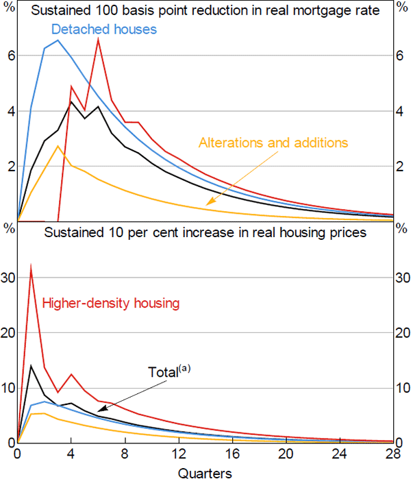
- Interest rates have a large and highly significant direct effect on construction activity, as might be expected from Figure 3 (top panel). Figure 4 (top panel) shows responses of approvals to a sustained[3] change in interest rates, holding real housing prices and income constant.
Notes:
Partial equilibrium responses
(a) Weighted by shares in national accounts dwelling investment
- The strong and clear response of residential construction to interest rates is evidence of the potency of monetary policy. It contrasts with the weak and imprecise response of other components of GDP. Researchers have had difficulty in finding an effect of interest rates on consumption, government spending, business fixed investment or inventories (e.g. Caballero 1999). In structural macroeconometric models (e.g. Brayton and Tinsley 1996; Powell and Murphy 1997; Treasury 2001; Fair 2004) effects of interest rates on other expenditure categories are often small or constrained. Consistent with this, structural macroeconometric models find that a large share of the effect of interest rates on GDP reflects dwelling investment[4], and research on the effects of monetary policy can usefully focus on the effects on housing.
- Real housing prices also have a large and highly significant effect on construction activity, as might be expected from Figure 3 (bottom panel). When the price of established housing increases relative to the cost of new housing, the incentive to build increases. Figure 4 (bottom panel) shows the estimated response, holding other explanatory variables constant.
- Although we describe our estimated responses to housing prices as large, estimates from Australian cross-section studies are much larger – often by several multiples. Examples include Gitelman and Otto (2012, Table 3), Liu and Otto (2014), McLaughlin (2011), McLaughlin, Sorensen and Glavac (2016), and Ong et al (2017, Section 3.3). Among other factors, we suspect this reflects differences between our time series estimates, which reflect decisions as to when to build, and cross-section estimates, which reflect decisions as to where to build. There seems to be much more substitution across space than across time.
- As shown in Figure 4 and Table 1, higher-density construction is much more sensitive to housing prices than are other components of dwelling investment. Gitelman and Otto (2012, Table 3) report similar results using census estimates of the housing stock. There are several possible reasons for this.[5]
- It is changes in interest rates and in existing housing prices that drive construction, not their level. So the direct effects of these variables are temporary. Although discussions of dwelling investment often emphasise levels, our attempts to include these in the model did not fit the data. For example, the ratio of approvals to income has been below average over the past decade (Figure 2, bottom panel), even though the level of real interest rates has been unusually low and the relative price of established housing has been unusually high. Similar results and extended discussions are provided by McLaughlin (2011) for Australia and by Mayer and Somerville (2000) for the United States.[6] The latter argue that the superior explanatory power of changes in housing prices and interest rates arises because the level of real housing prices should match the dwelling stock with housing demand. Therefore, a permanent shift in the level of housing prices (or interest rates) would have a finite long-run effect on the level of the dwelling stock, and hence only a temporary effect on the level of net investment. Another interpretation is that these relationships reflect changing political pressures that tighten or loosen land use regulations.
- Other variables that might be thought to directly affect dwelling investment include the rate of economic growth, population growth, construction costs, depreciation, the price of vacant land, rents, long-term interest rates and the user cost of capital. However, most of these were statistically insignificant in our approvals equations. Others had the incorrect sign – perhaps because they proxied for omitted trends (see below). This is not to say that these variables are unimportant – it may just be that they showed little variation over our sample period. In contrast to Ball et al (2010, Equation 10b), Caldera and Johansson (2013, Table 2A) and IMF (2018), we did not find the ratio of established housing prices to the cost of new housing, or Tobin's q, to be significant. The insignificance of the q-ratio may be because the change in existing housing prices captures most of its effect and because the cost of new houses and land is poorly measured.[7]
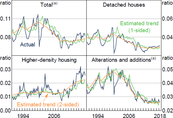
- While the ratio of dwelling investment to income seems to have been roughly stationary over the past 60 years, it is not precisely constant. Gradual changes in this ratio are likely due to omitted variables, such as the q-ratio, foreign investment, taxes, zoning regulations, chain aggregation and expectations of future demand. These variables are more difficult to quantify than the variables noted in the previous dot point, so it is harder to dismiss their importance. Moreover, shifts in the composition of housing from low to high density will also affect the component-level estimates of the approval-to-income ratios. To account for factors like these, we allow the intercepts in our models to change gradually over time. These can be interpreted as time-varying ratios to disposable income, shown in Figure 5. The use of time-varying intercepts is supported by coefficient stability tests for OLS versions of Equation (1); Quandt-Andrews exp-F tests of stability of the intercept have p-values of 0.6 per cent for detached houses, 0.8 per cent for higher-density housing and 11 per cent for alterations and additions.
Note: (a) Alterations and additions have been scaled to be representative of their share of dwelling investment
Sources: ABS; Authors' calculations; RBA
4.2 Other Construction Variables
Our model contains a detailed set of equations that trace out the lags in the construction process. Building approvals feed into two separate but related chains of variables, which estimate:
- constant price measures of housing construction, which are predominately used for estimates of dwelling investment and the real value of the housing stock, and
- the number of new dwellings, which feeds into estimates of the rental vacancy rate.
The translation from approvals to the number or value of dwellings is complicated by timing lags, changes in quality, demolitions and other factors. However, these details are mainly of interest to specialists. We briefly mention some key results below and discuss the details in Online Appendix B. The estimated equations are E4–E16 in Online Appendix E.
4.2.1 Dwelling investment and the housing stock (constant prices)
Dwelling investment is a volatile component of GDP(E) and is important for macroeconomic forecasting and policy. It has also been a focus of other researchers and model builders, so our predictions for it facilitate comparisons. Approvals flow into dwelling investment with a long-run elasticity of 1. Specifically, for each category of housing construction, we map approvals through to commencements, then commencements to work done, work done to dwelling investment, and finally, dwelling investment to the constant price measure of the housing stock.
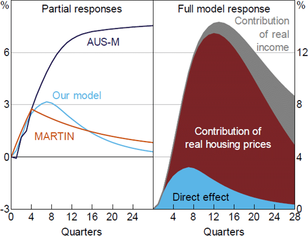
Figure 6 shows our estimated response of dwelling investment to real interest rates. The left-hand panel shows partial responses, holding housing prices, income and other variables constant. These results are directly comparable with the top panel of Figure 4. Comparable results are also shown for two leading Australian macroeconomic models, the AUS-M model of Outlook Economics and the RBA's MARTIN model (with thanks to Adam Hamilton). Over the first year, responses are essentially the same. AUS-M (like its predecessor TRYM) has larger long-term effects because its specification assigns a large persistent role to the level of interest rates, a point discussed above. For an overview of dwelling investment in AUS-M and TRYM, see Jovanoski et al (1997, Section 4.3).
The right-hand panel shows full model responses. In addition to the direct effect (blue), reproduced from the left-hand panel, this includes effects working through housing prices (dark red) and income (grey). The peak full effect is about four times as large as the direct effect, largely reflecting effects working through housing prices. AUS-M and MARTIN also show large effects through housing prices, though the magnitude of differences is sensitive to precise details of the experiment. Coupled with footnote 4, this implies that one of the largest channels through which interest rates affect real GDP is through housing prices. This experiment makes the important assumption that the change in interest rates is expected to be sustained, so flows through fully into long-term interest rates and the user cost of housing. If long-term rates did not change, the estimated contribution from prices would be much smaller, peaking at about 2½ per cent of dwelling investment. The relationship between interest rates and housing prices is discussed in Section 4.5.
Sources: Authors' calculations; Outlook Economics; RBA
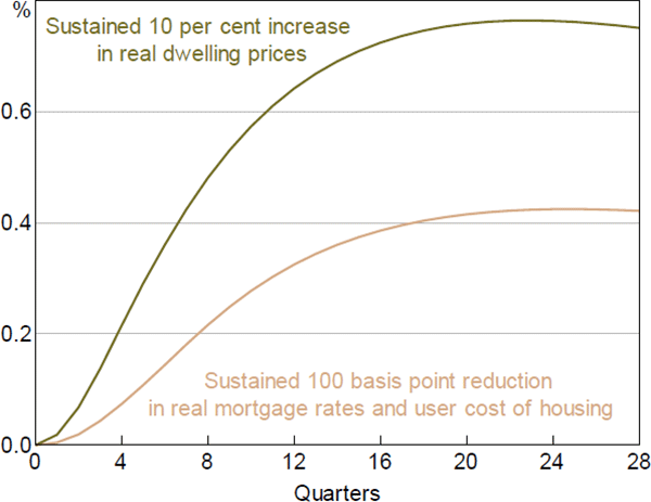
Coupled with (exogenous) depreciation, accumulated investment determines the stock of housing. The lighter line in Figure 7 shows partial responses of the housing stock to a sustained percentage point decrease in real interest rates, holding housing prices, incomes and other variables constant. This increases the housing stock by 0.4 per cent after four years.
As shown by the darker line in Figure 7, a sustained 10 per cent increase in real dwelling prices, holding interest rates, incomes and other variables constant, raises the constant price measure of the housing stock by about 0.7 per cent. This peak elasticity of 0.07 is substantially below estimated price elasticities of 0.4 for Sydney property by Gitelman and Otto (2012, Table 3) or 0.3 for regional NSW property by Liu and Otto (2014). As noted earlier, we suspect much of this difference represents a difference between time-series and cross-section studies. The contrast is even larger for studies such as Ball et al (2010) and Caldera and Johansson (2013) that find the level of prices permanently affects investment, which would make the long-run effect on the housing stock infinite (in the absence of depreciation).
It is often suggested that increased subsidies or tax concessions for housing would have little effect on supply, which is said to be constrained by limited land and planning permissions. That view seems to be inconsistent with the responsiveness to relative prices that we and others estimate. Although our estimates are smaller than others, they are still significant. Legal and physical restrictions on land development are important, but they appear to be either responsive to financial considerations or not fully binding.
The housing stock plays an important role in some models of the housing market. For example, feedback from the stock can help explain ‘cycles’ or oscillations in construction (Jovanoski et al 1997, Section 2.1). However, we were unable to find a satisfactory role for the housing stock in our equations. The housing stock is highly correlated with income and fits the approvals data slightly better. However, our judgement was that the high correlation between construction and income is an important feature of the data and it was difficult for a model with a large role for the housing stock to capture this. As discussed below, the number of dwellings seems to matter for balance in the rental market. But the size and quality of those dwellings does not. As we show in Section 5, our model does not exhibit important ‘cobweb’ or oscillatory responses. Berger-Thomson and Ellis (2004) find that the cyclicality in dwelling investment reflects cyclicality in interest rates.
4.2.2 Completions and the number of dwellings
The second chain of variables affected by dwelling approvals explains the number (as distinct from the value or volume) of dwellings that are built. As discussed in more detail in Online Appendix B, to estimate the number of approvals we remove alterations and additions and the effect of the changes in quality (most evident in larger floor sizes) from the estimates of new dwelling approvals discussed in Section 4.1. We then map the number of new approvals through to the number of commencements, then commencements to completions, and completions to the number of dwellings, which feeds into estimates of the rental vacancy rate. For both detached houses and higher-density housing, approvals flow through to completions with an elasticity of 1, although with different lags. We estimate that 83 per cent of detached houses are completed one year after approval, and 95 per cent in the long run. For higher-density housing, 61 per cent of approvals are completed within a year and 85 per cent in the long run.
In simulations below, the number of dwellings typically reacts substantially less to shocks than does the constant price measure of the housing stock. As this implies, the average quality of dwellings plays a large part in responses. That partly reflects changes in alterations and additions, which affect the constant price stock, but not the number of dwellings. It is also because dwellings built now are of a higher quality than those in the current stock. So new construction increases the average quality.
As discussed in Online Appendix B, we assume that the average quality of new dwellings is proportional to income per capita. This implies that, while constant price approvals and residential investment are proportionate to total income in the medium run (Section 4.1), the number of approvals and completions is proportionate to population. Hence, in steady state, they grow at the same rate.
4.3 Rental Vacancies
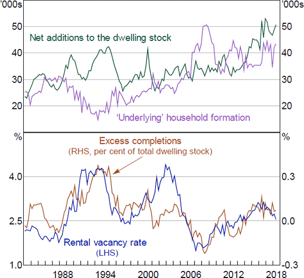
Figure 8 shows components of what might be considered as ‘excess supply’ of housing. The green line in the top panel shows quarterly changes in the number of dwellings. This equals housing completions (as modelled in the previous section) less demolitions.[8] This is often called the supply of new dwellings, though the demand/supply distinction is difficult to apply to owner-occupied housing, which households provide to themselves. These estimates are lower than the ‘housing supply’ estimates of Ong et al (2017, Section 2) because we allow for both approvals that are not completed and demolitions. The purple line shows what we call ‘underlying’ household formation, defined as quarterly changes in adult population, which is an important and exogenous component of underlying demand, divided by a five-year trailing average of adults per dwelling.[9]
We refer to the gap between these series as ‘excess completions’ measured as
where K is the total number of dwellings, WAP is working-age population (15+), and is the five-year trailing average of adults per dwelling. Excess completions are plotted as the brown line in the bottom panel of Figure 8, as a share of the total number of dwellings. This resembles, though is somewhat simpler than, the ‘housing gap’ measure examined by Kohler and van der Merwe (2015) or the ‘State of Supply Reports’ of the National Housing Supply Council (e.g. NHSC 2014).
Sources: ABS; Authors' calculations; Real Estate Institute of Australia (REIA)
The blue line in the bottom panel shows the rental vacancy rate, measured as the number of properties listed as available for rent, divided by the total number of rental properties. As shown in the figure, excess completions and the vacancy rate move together closely. This is perhaps not surprising given that both series can be interpreted as measures of excess supply in the housing market. Despite these considerations, researchers have not been able to successfully model this relationship. See, for example, the discussion in Jovanoski et al (1997, p 9). That is partly because the vacancy rate is a stock whereas excess completions are a flow and partly because the high-frequency correlation between the series is very weak.
Observation of local housing markets suggests that the relationship between excess completions and the vacancy rate is causal. When extra households are formed, for example due to higher immigration, the market tightens and vacancies fall. When extra stock comes onto the market following a building boom, vacancies rise. Accordingly, we assume that excess completions drive the vacancy rate. However, we assume that they do so gradually, so that the correlation evident in Figure 8 holds in the long run, but not instantaneously. Moreover, we add the change in the unemployment rate and reversion to the mean, both discussed below. Specifically:
where V is the rental vacancy rate, EC is excess completions, K is the total number of dwellings, UR is the unemployment rate and White t-statistics are in brackets. Detailed estimates are at equation E17 in Online Appendix E.
The change in unemployment represents the effect of the business cycle: extra employment and income increase demand for housing and reduce desired household size. Ideally, these effects – like reversion to the mean – would be captured by changes in household size and hence as an additional determinant of household formation. In practice we are unable to distinguish these changes in household size from those that endogenously accompany and neutralise building completions. As an expedient, we fix the number of adults per dwelling at its previous five-year average and allow factors that affect household size to enter Equation (2) directly. Although this complicates the interpretation, these variables have high explanatory power, as judged by the t-statistics in Equation (2).
The estimated steady-state vacancy rate – at which the vacancy rate has no tendency to change – is a function of excess completions. When excess completions are zero, so the number of dwellings is increasing as quickly as underlying household formation, the steady-state vacancy rate would be 2.4 per cent. This benchmark corresponds to some interpretations of ‘balance’ in the housing market and we use it in our equation for rents. However, other benchmarks are also interesting. To stabilise vacancies at their historic mean, 2.8 per cent, would require excess completions of 0.06 per cent of the housing stock per quarter. A vacancy rate of 3 per cent would keep rents growing at the same rate as other consumer prices; this would require excess completions of 0.09 per cent of the housing stock per quarter.
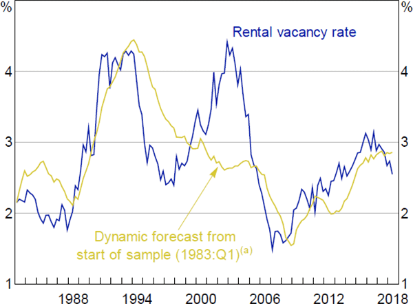
The short-run contribution of excess completions is not estimated but constrained to a value that seems plausible and provides reasonable system properties. Specifically, new completions increase the number of rental vacancies in proportion to the share of rental accommodation in the housing stock, which was 29 per cent at the time of the 2011 ABS Census. That is, if the total housing stock increased by 100 dwellings, the number of vacant rental properties would initially increase by 29 dwellings. Although the short-term fit of this equation is not good, the model does explain longer-term variations in vacancies, as judged by a dynamic simulation starting from 1983:Q1 (Figure 9) and model simulations discussed in Section 5. Moreover, combined with other equations, the overall system has similar properties to a reduced-form regression in which growth of real rents is directly explained by excess completions (not shown) or studies of the effect of housing supply on prices (Section 5.3).
A limitation of our model is that we assume that household formation is largely a function of exogenous population. This means that imbalances in the housing market are corrected by adjustments to supply, not demand. The assumption that population growth is exogenous seems reasonable (overseas arrivals are cyclical, but feedback from the housing sector is small). However, household size surely responds to price signals. In preliminary work, we estimated that rising real rents have increased the number of adults per dwelling since the early 1980s, but this effect has been more than offset by higher real incomes. However, this result was highly sensitive to the chosen model specification and sample period. This is an issue for future research.
Note: (a) The forecasts use actual data for the explanatory variables
Sources: Authors' calculations; REIA
4.4 Rents
Our equation explaining the growth of real rents is as follows:
where rent is real CPI rents, V is the rental vacancy rate (entered as the deviation from its benchmark value of 2.4), and Δinc is the growth in real household disposable income (measured as the deviation from its sample mean). Rents and income are in logs and deflated by annualised trimmed mean CPI inflation over the previous three years. βi, αi and ϕi are lag weights, each of which sums to 1. White t-statistics are in brackets. Detailed estimates are at equation 18 in Online Appendix E.
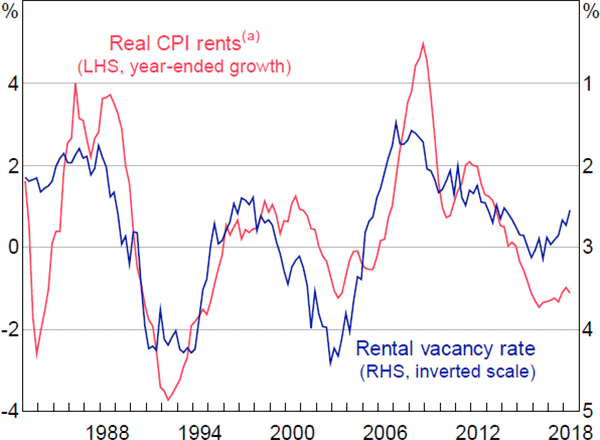
The dominant influence on real rents is the vacancy rate, as shown in Figure 10. This effect is analogous to the Phillips curve in the labour market. However, whereas the Phillips curve seems increasingly difficult to see (Gillitzer and Simon 2015), the effect of an excess supply of housing on changes in rents is clear, with the coefficients on the vacancy rate in Equation (3) being highly significant.[10] It is sometimes questioned whether the balance of supply and demand affects the cost of housing (Phibbs et al 2017; Coates 2018), but the evidence seems to be strong.
Note: (a) Deflated by annualised growth of trimmed mean CPI over the previous three years
Sources: ABS; Authors' calculations; RBA; REIA
When the vacancy rate is 2.4 per cent, the rate consistent with the housing stock increasing as fast as population, real rents are estimated to grow at 0.9 per cent a year. The vacancy rate will deviate from this benchmark due to changes in population growth, underlying household size, zoning regulations and so on. Any projection of rents, housing prices or other features of the housing market requires an assessment as to how these factors will evolve, which our model does not explore.
Rents exhibit a high level of momentum, with coefficients on the lagged changes in real rents summing to 0.7 (standard error = 0.06). This inertia, coupled with the high explanatory power of the equation (R 2 = 0.80), makes rents unusually easy to forecast, relative to other components of the CPI.
Equation (3) resembles that of Jovanoski et al (1997, Section 4.1). The main difference is that we smooth non-rental prices by averaging over time rather than by controlling for import prices. Neither the real nor the nominal share of rent in consumption or income, nor the relative price of rent have been stationary. So we do not impose these as long-run conditions.
4.5 Housing Prices
Research on the determinants of housing prices, both in Australia (Otto 2007; Abelson 2018) and overseas (Duca, Muellbauer and Murphy 2011; Glaeser and Nathanson 2014; Oxford Economics 2016), commonly focuses on the user cost of housing. The user cost represents the annual cost of owning a house, comprising the sum of interest payments, repairs, rates and other running costs, less expected capital appreciation. For recent Australian estimates and discussion, see Fox and Tulip (2014).[11] In the long run, this tends to be close to the cost of renting a similar dwelling. If the user cost were lower than rents, households would be financially better off owning than renting and might be expected to bid up the price of houses. Conversely, when renting is cheaper, there would be downward pressure on housing prices. This implies the arbitrage condition:
where USERCOST is the user cost of housing expressed as a share of the dwelling value. In our estimated equation, housing prices gradually adjust to this long-run target so as to keep the cost of owning close to the cost of renting. In the short run, prices exhibit strong momentum and respond to short-term variable rates. Specifically:
where dp is real dwelling prices, rent is real CPI rents, usercost is the user cost of housing, and R is the real discounted variable mortgage rate. Lower case variables are in natural logs (so rent – dp is the log of the rental yield). Housing prices and the mortgage rate are deflated by annualised trimmed mean CPI inflation over the previous three years. White t-statistics are in brackets. Detailed estimates are at equation E19 in Online Appendix E. Otto (2007) finds that similar specifications explain city-level changes in house prices in Australia.
The gradual adjustment of the rental yield towards the user cost and the momentum in short-term price movements make housing prices quite predictable. Our equation has an R 2 of 0.69, with no contemporaneous regressors. The predictability of changes in housing prices is well established (Case and Shiller 1989; Glaeser and Nathanson 2014). It is also inconsistent with models of efficient asset pricing, in which predictable movements are arbitraged away. One possible interpretation of the large coefficient (0.74, t = 11) on the lagged change in prices is that it reflects extrapolative expectations, which could make the market prone to bubbles. Another interpretation is that it reflects gradual adjustment to omitted variables.
However, any deviations from efficiency appear to be transitory. In the long run, prices move towards their efficient level given by Equation (4). One implication is that a change in rents is fully reflected in a change in housing prices, though this takes many years to flow through.
Our estimates of the user cost assume that expectations of capital gains are exogenous and approximately constant, equal to the historical mean. These expectations are simple, naïve and involve an inconsistency: market participants will bid up housing prices on the implicit assumption that other buyers will behave differently. More complicated assumptions are easy to imagine but fit the data less well.[12] As discussed in Section 5.4, our assumption of mean expectations is quite different to model-consistent expectations. However, it is unclear how expectations should be modelled. In the long run, it would be desirable if expectations were consistent with the model, though the literature on housing bubbles suggests that model-consistent expectations are an unrealistic assumption in the short run.
User cost models like ours differ from reduced-form models in which housing prices are directly determined by fundamentals such as housing construction or population.[13] As shown in Section 5, variables like these have large effects on housing prices in our model, but they do so indirectly by affecting the balance of demand and supply of housing as measured by vacancies and changes in rents. One advantage of our approach is that it directly maps into the decisions of home buyers, who will take rents and the user cost as given. Reflecting this, user cost models provide a relevant measure of ‘overvaluation’ that can be used in household financial decisions and in detecting bubbles, as argued by Fox and Tulip (2014).[14] Another advantage is that our approach is more comprehensive. If some factor were to boost the demand for housing, but this effect was offset by higher supply, so that vacancies and rents do not change, there should be no effect on house prices. Controlling directly for rents allows all factors determining demand and supply – including those the econometrician does not observe – to enter. Weaknesses of our approach would be if our estimates of rents and the user cost were mismeasured or if fundamental factors affected future but not current rents. Empirically, those problems do not seem to be important. When added to Equation (5), these other variables are not statistically significant over our sample period.
The effect of interest rates on housing prices plays an important role in several of this paper's conclusions and is somewhat complicated. So the effect and the evidence of its strength are worth explaining.
At a user cost of 6 per cent we estimate that a sustained percentage point drop in interest rates would, in the long run, boost housing prices by 17 per cent, holding rents and other components of the user cost equal. This semi-elasticity (the proportionate increase in housing prices for a given percentage point increase in interest rates) is larger than the time series estimates of Abelson et al (2005), perhaps because they control for many other variables affected by interest rates (e.g. share prices and income), so only capture part of the effect of interest rates. Our estimate is similar to Gitelman and Otto's (2012, p 183) estimate of 20 per cent for Sydney housing prices using disaggregated census data, and Himmelberg, Mayer and Sinai's (2005, p 78) estimated range of 19 to 33 per cent for the United States in a calibrated model.
A user cost (or rental yield) of 6 per cent is the approximate average over Gitelman and Otto's sample. User cost models, such as Equation (4), imply that the semi-elasticity increases as the user cost declines.[15] Effects on prices become extremely large as the denominator in Equation (4) approaches zero. With a current user cost of 3½ per cent (well below that observed in the studies above), a percentage point drop in the expected real mortgage rate would boost housing prices by 28 per cent in the long run.
These large effects reflect cointegration between the rental yield and the user cost (Equation (4)). Our estimates of Equation (5) (E19 in Online Appendix E) and textbook models of asset pricing both support this assumption, but we would not describe this evidence as strong. While the coefficient on the error correction term is statistically significant (t-statistic of 2.6), it is small (0.023) and sensitive to alternative specifications.
Stronger evidence in favour of Equation (4) is its ability to explain the level of prices. According to CoreLogic, the average rental listing for houses across seven capital cities in August 2017 was $24,000 a year.[16] Divided by the September quarter 2017 user cost of 3.6 per cent, Equation (4) implies home buyers would be as financially well off paying $667,000 for a similar dwelling. This is close to CoreLogic's estimated valuation of those same rental properties of $735,000.
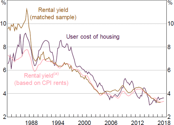
This comparison can be repeated at earlier dates, as shown by Figure 11, which shows the user cost of housing and two estimates of the rental yield. The brown line uses CoreLogic data on matched samples, where rents and imputed prices are measured for the same properties. As Fox and Tulip (2014) argue, this is a relevant measure for explaining housing prices and their ‘fair value’. The CoreLogic series is available from 2005 to September quarter 2017. Before 2005 we splice with REIA estimates of median rents and prices, which are not matched but use consistent definitions. Both the level and low-frequency changes in this measure of the rental yield match the user cost – especially in the latter part of the sample, when data quality is higher. Close long-term relationships between alternative measures of the user cost and the rental yield are also shown for Australia by Otto and Stapledon (2017, Figure 2) and for the United States by Duca et al (2011, Figure 2).
Note: (a) Scaled to have same mean as the matched sample rental yield from 1988 to 2018
Sources: ABS; Authors' calculations; Corelogic; REIA
Our model uses more widely known and accessible series for rents and prices: the rent component of the consumer price index and the CoreLogic hedonic price index. The ratio of these series is shown as the pink line in Figure 11. In contrast to the matched sample, these series are in different units, so they do not explain the level of housing prices, however, they still explain longer-run variations. We have adjusted the mean of their ratio to equal the matched sample rental yield from 1988 to 2018. In principle, different quality adjustments in the numerator and denominator of this measure of the rental yield make its longer-term movements difficult to interpret. In practice, the correspondence of this series to the matched sample estimate suggest this inconsistency has not been important.
It is the path of interest rates expected over the ownership of the asset that determines the full cost of purchase. So long-term interest rates enter the user cost. However, housing prices seem to also respond to variable mortgage rates in the short run, possibly because of cash flow constraints. To account for this, we have included changes in the real variable mortgage rate in Equation (5).
Short-run responses will depend on how long a change in interest rates is expected to be sustained and on how quickly this is reflected in long-term interest rates. Modelling expectations is outside the scope of this paper. However, in Section 5.1 we consider a percentage point cut in interest rates that is expected to be sustained for three years, which may be representative. In this scenario, dwelling prices increase by 8 per cent after two years. This estimate is near the middle of the range of estimates surveyed by Williams (2016, Table 1).
To summarise, although our estimated responses of housing prices to interest rates may seem surprisingly large, they are in line with other research (both in Australia and overseas), and are consistent with theory and the available data.
Since 1982, real dwelling prices have grown at an average annual rate of around 3 per cent, approximately tripling in value (depending on the measure). About 18 percentage points of this increase is attributable to the increase in real rents over this period. The substantial majority of the change represents a decline in the rental yield, which as Figure 11 indicates is essentially explained by the fall in the user cost. Most of this fall reflects a decline in expected real mortgage rates from a peak of 6 per cent in the 1980s to 3.2 per cent recently. Holding rents and other components of the user cost constant, this would account for a 45 per cent increase in housing prices. Other components of the user cost, in particular running costs, also contribute. However, reflecting the nonlinearity discussed above, the interaction of these components is more important than any other single contribution. Moreover, reflecting volatility of bond yields in the early 1980s, any quantitative decomposition is quite sensitive to the assumed starting point.
This explanation of the trend increase in housing prices differs from other popular accounts. It is straightforward to reconcile some of these:
- Other factors that raise demand for housing, such as immigration or income growth, boost prices by raising rents, which the implicit counterfactual above takes as given. When this assumption is relaxed – as in Section 5.2, for example – these demand-side factors have large effects on prices.
- Kendall and Tulip (2018) attribute higher prices to zoning regulations. In terms of a conventional supply-demand diagram, zoning restrictions make the supply curve steep, while lower interest rates (or other factors) shift the demand curve out. It is the interaction of rising demand with inelastic supply that explains higher prices.
- The liberalisation of credit markets, emphasised by Yates (2011, Section 2.2) among others, led to a narrowing in lending margins. This is a significant factor in the large decline in real mortgage interest rates over this period.
- According to the Taylor principle, nominal interest rates should respond more than one-for-one to deviations of inflation from target. Hence the change in inflation from above target at the beginning of our sample to below target recently accounts for some of the downtrend in real interest rates.
In contrast, our model would need to be modified to allow for some other suggested explanations of the boom in house prices.
- Anecdotal observation, the important role of variable rates and previous RBA work (see the references in RBA (2014, p 6)) suggest, without quantifying, that changes in borrowing limits affect housing prices in the short run. For example, tightening in lending limits seems to be important in the decline in house prices in 2018. Some international research (e.g. Duca et al 2011) finds a larger role. However, Australian empirical research, such as Otto (2007) or our investigations, has not found borrowing limits to have longer-run effects on house prices. Borrowing constraints affect the demand for housing assets not the demand for housing services. As Kaplan, Mitman and Violante (2017) discuss, this would be expected to affect the ownership rate, not the level of house prices.[17]
- Our measure of the user cost is relevant to owner-occupiers. A more complicated measure for investors would be needed to assess the effect of tax changes. This is a task for future research. Daley, Wood and Parsonage (2016, Box 6) estimate that the concessional treatment of capital gains tax and negative gearing may boost the level of housing prices by about 2 per cent.
4.6 Other Equations
The full model contains 62 equations, presented in Online Appendix E. Most of these are identities or autoregressions. However, three further equations might be worth mentioning. Our equation for real income is calibrated so that it reflects the response of GDP to the real cash rate in the MARTIN model.[18] The unemployment rate reacts to income in line with Okun's rule. Long-term interest rates (which feed into the user cost) equal the average of future variable rates.[19]
Footnotes
The Australian Bureau of Statistics (ABS) measure of building approvals (ABS Cat No 8731.0) is based on local council building permits. It should not be confused with development approvals, which typically occur months or even years earlier. [1]
For these and other figures, variable definitions and sources are given in Online Appendix D. [2]
By ‘sustained’ we mean that the shock lasts for at least as long as the effects that are shown and long-term interest rates move by the same amount as short-term rates. It is tempting to describe this change as ‘permanent’, except that permanent shifts in interest rates are not feasible in many macroeconomic models. [3]
In our simulations of the AUS-M model of the Australian economy, about half the effect of interest rates on GDP comprises dwelling investment. Unpublished simulations of MARTIN by Tom Cusbert find that housing accounts for about 30 per cent of the total response. Estimates for other countries seem to be somewhat smaller (e.g. Mishkin 2007), though consistent comparisons are difficult. As Paul Krugman (2014) writes, ‘one of the dirty little secrets of monetary policy is that it normally works through housing, with little direct impact on business investment’. [4]
One possibility is that changes in the price of existing dwellings largely reflect land prices. When land prices increase, higher-density housing becomes more attractive. Another possibility is that higher-density housing is more flexible than detached housing, which often requires land release and neighbourhood planning. However, it is difficult to reconcile these explanations with how quickly higher-density approvals respond. A more important factor may be variations in the availability of finance. This is because the sequential timing of cash flows for large developments makes their equity position quite sensitive to near-term price movements. [5]
As we show in Figure 6 below, interest rates also have only temporary direct effects on the level of dwelling investment in the MARTIN model. However, once effects on other expenditure components and their interactions are allowed for, MARTIN finds that interest rates have highly persistent effects on real GDP growth. So, while it is the change in interest rates that matters for dwelling investment (as a short-run approximation), it is the level of interest rates that matters for overall economic growth and the integral that matters for the level of overall activity. [6]
We are unaware of any aggregate time series data on the cost of new houses that includes land costs. The series we used for these exercises were constructed using ABS data on the cost of building new houses and data from a number of sources on land prices. [7]
Demolitions are estimated as the interpolated difference between accumulated completions and the census estimate of the number of dwellings. In projections, they are assumed to be a constant 8 per cent of completions. See Section B.3 in the Online Appendices for more details. [8]
Actual household size is highly endogenous, adjusting so as to keep demand and supply in approximate balance, so lacks predictive power. [9]
A percentage point increase in the vacancy rate reduces the annual growth of real rents by 2 percentage points initially and by 1.4 percentage points (= 0.001 x 400 / (1 – 0.72)) in the long run. [10]
Following Fox and Tulip (2014, Equation (2)), we define the user cost as:
where c is running costs; s is transaction costs; and d is the physical depreciation rate. After 2014, these are held constant. π is the expected real appreciation rate, assumed to equal its post-1955 mean. r is the average real expected variable mortgage rate, which Fox and Tulip estimated using 10-year fixed mortgage rates. However, subsequent data and analysis suggest that expected interest rate changes can be more reliably estimated from the yield curve on government bonds. From 1997 r is estimated as:
where vmr is the (package or average discounted) variable mortgage rate for owner-occupiers, bond is the 10-year government bond yield, cash is the cash rate, inflation is 10-year inflation compensation derived from indexed bonds and the superscript bar represents the sample mean, used to remove the average term premium from the yield curve. The average discounted rate is publicly available from 2005, prior to which we splice to the standard variable mortgage rate. Variable mortgage rates have closely followed the cash rate since 1997, but before then were noticeably less volatile. From 1982 to 1997, we assume the expected variable mortgage rate is a constant spread (equal to its 1997 level) to the 10-year government bond yield.
[11]The simplest alternative would be to assume lower expectations and include a constant ‘ownership premium’. This would be observationally equivalent. [12]
For examples of such reduced-form models, see Bourassa and Hendershott (1995), Abelson et al (2005), Caldera and Johansson (2013), Tumbarello and Wang (2010), and IMF (2018). [13]
Our most recent data, for June quarter 2018, imply that if prices are expected to grow at the same pace as in the past, then renting is about as expensive as buying (the user cost and the rental yield are both 3½ per cent), and hence that houses are fairly valued. If prices were expected to grow slower, as implied by our forecast in Online Appendix C, houses would be overvalued. We discuss further in Section 5.4. [14]
The semi-elasticity equals the inverse of the user cost, which in equilibrium will equal the price-to-rent ratio. See Fox and Tulip (2014, Equation (9)). [15]
This is the most recent period for which we have matched data. Estimates are seasonally adjusted and rounded. [16]
The RBA (2018) finds that borrowing limits are typically not binding. [17]
A sustained 1 percentage point reduction in the real cash rate raises the level of income by about 1.8 per cent after two years and about 3.7 per cent after five years. Thanks to Adam Hamilton for these estimates. [18]
Specifically, the 10-year government bond yield is the geometric average of the path for the cash rate over the coming ten years, which in our baseline projections follow zero-coupon forward rates. [19]