RDP 2016-02: Disagreement about Inflation Expectations 4. Descriptive Analysis
April 2016
- Download the Paper 1.07MB
4.1 Professional and Union Surveys
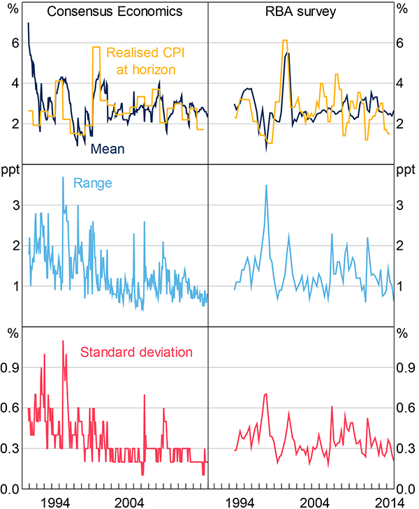
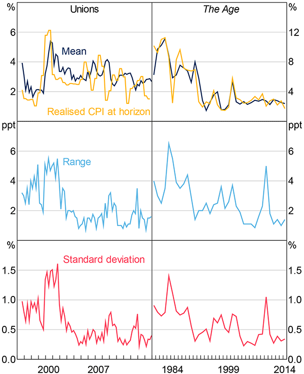
Figures 1 and 2 plot the mean, range, and standard deviation of responses for each survey measure of inflation expectations, except for the consumer measure. The consumer measure has several unique features and is discussed in the next section. We present two measures of disagreement: the range of responses (highest minus lowest response in each survey), and the standard deviation of responses. We prefer the standard deviation measure because it is more robust to a single extreme survey response than the range, but in general the information conveyed by each measure is qualitatively similar.
Note: The standard deviation of responses to the Consensus Economics survey is reported to one decimal place
Sources: ABS; Authors' calculations; Consensus Economics; RBA
Note: End-of-year survey data from The Age reported
Sources: ABS; The Age; Authors' calculations; Workplace Research Centre
The first notable feature of the data is a decline in the level of disagreement for each of the surveys during the 1990s, which supports the idea that inflation expectations have become better anchored. A reduction in disagreement is most evident in The Age survey, the only measure for which individual response data is available for the 1980s. The standard deviation of responses to The Age survey averaged around 0.9 per cent over the 1980s, compared to 0.4 per cent over the past decade. Some decline in the average level of disagreement is also apparent for the Consensus Economics measure, with the standard deviation of responses averaging around 0.6 per cent in the early 1990s – when inflation targeting was in its infancy – and around 0.2–0.3 per cent more recently.
Second, there is clear time variation in disagreement for each of the survey measures. This variation is also somewhat common to the different measures; the degree of co-movement in disagreement between the series is reported in Table 3, which reports correlations for the quarterly Consensus Economics (end-of-quarter monthly survey), RBA and union survey measures (The Age survey is not available on a quarterly basis). The presence of co-movement suggests that the variation in disagreement through time is not just noise, but is economically meaningful.[3] In terms of the models discussed in Section 2, the mere existence of disagreement is inconsistent with the FIRE model, and time variation in disagreement is superficially inconsistent with the baseline noisy-information model, which does not generate variation in disagreement absent changes in the signal-to-noise ratio of economic data available to forecasters.
| Consensus Economics | RBA survey | Unions: year-ahead | Unions: medium-term | |
|---|---|---|---|---|
| Consensus Economics | 1 | |||
| RBA survey | 0.39 | 1 | ||
| Unions: year-ahead | 0.37 | 0.31 | 1 | |
| Unions: medium-term | 0.37 | 0.20 | 0.81 | 1 |
| Notes: Contemporaneous correlations using standard deviations of year-ahead inflation forecasts for the period 1996–2014; we do not report a correlation for The Age survey measure here because it is not available quarterly | ||||
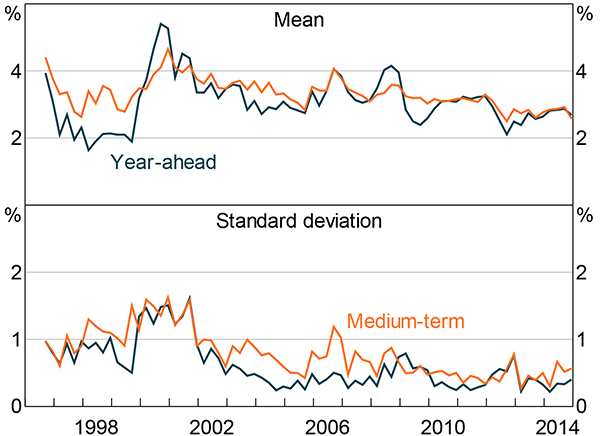
Third, co-movement of disagreement is also very strong between the short- and medium-term measures of inflation expectations in the union survey. If expectations are rational and well-anchored, transitory deviations in short-term expectations should have little effect on medium- and long-term expectations, resulting in a low correlation between the measures. In contrast, the strong correlation between disagreement in short- and medium-term expectations provides some evidence against well-anchored inflation expectations. In addition, there is a strong correlation between short- and medium-term expectations at the individual union level, indicating that when short-term expectations are revised there is a flow-on effect to medium-term expectations. This suggests that it is reasonable to make inference about the anchoring of inflation expectations from a dataset principally limited to short-term measures. Interestingly, disagreement among union officials has almost always been higher for medium-term than short-term inflation expectations (Figure 3).
Sources: Authors' calculations; Workplace Research Centre
As discussed in the introduction, one justification for relatively low inflation targets is that low levels of inflation are likely to be associated with low levels of uncertainty about inflation. Providing some support for this argument, there is tentative graphical evidence of a relationship between mean inflation expectations and disagreement (which is formally tested in Section 5.2). In the mid 1990s, and in the period leading up to the global financial crisis, realised and expected inflation was at an elevated level and so was disagreement. Co-movement between disagreement and inflation expectations is consistent with the sticky-information model, because only a fraction of agents revise their forecasts each period, and periods of elevated inflation are likely to be periods in which those updating their forecasts make relatively large changes.
The introduction of the goods and services tax (GST) in July 2000 is an interesting episode in light of the sticky-information model. For the union survey measure, there was a pronounced rise in disagreement when the GST was introduced. Despite respondents being explicitly asked whether their expectations incorporated the effects of the GST, several respondents did not incorporate the policy change into their expectations during this period, clearly showing inattentiveness. In addition, the range of estimates of the size of the ‘GST effect’ spanned around 5 percentage points, indicating genuine disagreement. For the other survey measures, there is no notable spike in disagreement around the time the GST was introduced, indicating that respondents to those surveys were attentive to the effect of the GST on CPI inflation and in broad agreement about its effect on the price level.
4.2 Consumer Survey
4.2.1 Raw data
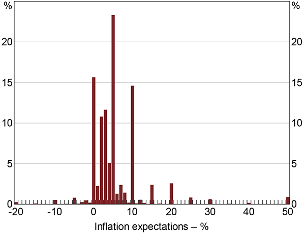
As mentioned earlier, the distribution of consumer inflation expectations exhibits characteristics that show a marked departure from those of professional forecasters. First, the distribution of consumer inflation expectations contains many more extreme values than the distribution of CPI inflation outcomes suggests is plausible. Responses of 50 and 100 per cent are given in most months the survey is conducted; well above the maximum observed CPI outcome of around 6 per cent since inflation targeting was introduced in 1993.[4] Thus, the distribution of consumer inflation expectations includes extreme values that cannot be explained by informed processing of available information. Extreme positive responses are more common than extreme negative responses, giving the distribution a positive skew. Second, and unlike for the professional survey measures, bunching of survey responses occurs at multiples of five. These two features of the data can be seen in Figure 4, which shows a histogram of responses to the consumer survey, pooled over the 1995–2014 period.
Note: Responses beyond axis limits attributed to bins at −20 and 50 per cent
Sources: Authors' calculations; Melbourne Institute of Applied Economic and Social Research
Measures of disagreement such as the standard deviation are sensitive to extreme observations. At the same time, extreme responses are likely to have little information content about ‘true’ community views, and will instead reflect other factors (Ranyard et al 2008; Bruine de Bruin et al 2010b).[5] For instance, it is possible that some respondents do not fully understand the concept of a percentage change or are not well informed about inflation developments. This could lead to responses that are selected at random, possibly at key round numbers, resulting in more instances of extreme observations.
Clustering at round numbers makes the distribution appear more discrete than continuous, with some large jumps in expectations between observations. However, assuming some respondents recognise their imprecision and thus round their expectations, these discrete responses can be thought of as representing a range of expectations centred on the particular number rather than a precise expectation. We would ideally like to observe a distribution that gives similar weight to observations around the cluster as the raw data, but that smooths out the distribution in between clusters.
In summary, some observations reflect accurate reporting of individuals' expectations of inflation, some are a discrete rounding of these expectations, while others are likely to represent noise with little information content. In order to ensure our analysis is robust, we use a structural framework to filter out noise and address bunching at round numbers.
4.2.2 Filtering the consumer inflation expectations data
Our approach imposes a categorical structure on the raw data, and then uses an ordered probit model to fit a normal distribution to the data. That estimated normal distribution provides the mean and standard deviation of inflation expectations, used in subsequent sections of the paper. The approach taken resembles that used by Bayer and Juessen (2015), who undertake a two-step analysis of ordinal data on self-reported wellbeing.
We believe this parametric approach is superior to the use of simple robust statistics, such as the median and interquartile range, as measures of the central tendency and disagreement in inflation expectations. While both the median and interquartile range measures impose less structure than our method, and are robust to extreme observations, they do not deal well with the clustering of expectations at round numbers.[6]
The disproportionately large share of responses equal to a multiple of five indicates that these observations likely reflect ‘rounded’ expectations. We allow for this by assuming that observations equal to a multiple of five reflect latent expectations in a small range above and below each multiple of five. For example, we assume the mass of reported inflation expectations at 5 per cent represents latent signals of future inflation over the interval 2.5 per cent to 7.5 per cent.[7] In contrast, there is little evidence of bunching at other points in the distribution, and we consider reported inflation expectations not equal to a multiple of five as ‘precise’.
The categorical structure we impose on the data before fitting an ordered probit model takes account of the distinction between rounded and precise observations. Because there are few observations not equal to a multiple of five outside the 0 to 10 range, we collapse all observations outside this range to the nearest multiple of five, limiting the number of categories for parsimony; we also fit only one category in the 6 to 9 range, centred at 7.5, owing to the few precise observations within this range. Lastly, we collapse observations within the range 32.5 to 100 (the maximum recorded value) and −12.5 to −50 (the minimum recorded value) into single bins.[8]
Table 4 reports the full categorical structure imposed on the raw inflation expectations data. The first column j reports the midpoint of each category (with the exception of the first and last category); the second column indicates whether the category represents a precise or rounded observation; the third column indicates the range over which latent signals for category j are assumed to be drawn; and the final two columns report the number and share of observations in each category for the period 1995–2014.[9] Note that the range for the rounded observations overlap the range for the precise observations within the 0 to 10 range.
| Midpoint: j | Type | Latent range | Number of observations | Share of observations |
|---|---|---|---|---|
| −15 | Rounded | −50 (min):−12.5 | 731 | 0.3 |
| −10 | Rounded | −12.5:−7.5 | 1,470 | 0.6 |
| −5 | Rounded | −7.5:−2.5 | 2,964 | 1.1 |
| 0 | Rounded | −2.5:2.5 | 41,352 | 15.7 |
| 1 | Precise | 0.5:1.5 | 5,463 | 2.1 |
| 2 | Precise | 1.5:2.5 | 26,881 | 10.2 |
| 3 | Precise | 2.5:3.5 | 30,888 | 11.8 |
| 4 | Precise | 3.5:4.5 | 14,085 | 5.4 |
| 5 | Rounded | 2.5:7.5 | 61,245 | 23.3 |
| 7.5 | Precise | 5.5:9.5 | 15,156 | 5.8 |
| 10 | Rounded | 7.5:12.5 | 41,087 | 15.6 |
| 15 | Rounded | 12.5:17.5 | 7,321 | 2.8 |
| 20 | Rounded | 17.5:22.5 | 7,092 | 2.7 |
| 25 | Rounded | 22.5:27.5 | 2,299 | 0.9 |
| 30 | Rounded | 27.5:32.5 | 1,674 | 0.6 |
| 35 | Rounded | 32.5:100 (max) | 3,213 | 1.2 |
The categorical structure just described allows for the bunching of observations at round numbers, but does not by itself adequately reduce the influence of extreme responses. To allow for extreme responses, we augment the ordered probit model with a uniform distribution from which noisy observations are assumed to be drawn. We estimate the relative weight on the ‘noise’ distribution and the latent underlying normal distribution from which ‘true’ expectations are assumed to be drawn.
Formally, our method proceeds as follows. First, we assign the raw data to the categorical bins
listed in Table 4; we use the notation  to refer to the
categorised inflation expectation of observation i. Second, we specify the
distributions from which ‘true’ and ‘noisy’ observations are assumed to
be drawn: ‘true’ observations are drawn from a normal distribution with mean
μ and standard deviation σ, and ‘noisy’ observations are
uniformly distributed over the range −50 to 100. The parameter ρ, which we
estimate, represents the proportion of true observations in each category. These assumptions are
summarised by Equations (1)–(3):
Third, we estimate the parameters ρ, μ, and σ by numerically maximising the log-likelihood function for cross-sections of reported inflation expectations.[10] Conditional on these parameters, the likelihood that a response to the inflation expectations survey lies within category j is given by:
where Φ is the cumulative standard normal distribution and UBj and LBj are the upper and lower bounds of category j, as detailed in Table 4. Figure 5 shows the categorical data and fitted distributions for inflations expectations data pooled over the 1995–2014 period.
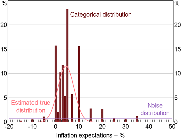
Sources: Authors' calculations; Melbourne Institute of Applied Economic and Social Research
4.2.3 Filtered data
The model's estimated parameters are shown in Figure 6, at a monthly frequency. Over time, about 5 to 10 per cent of the distribution is classified as ‘noise’, and so in effect purged when estimating the underlying parameters of the data. As a result, the true underlying distribution is estimated to be tighter as the extreme values no longer distort the results.
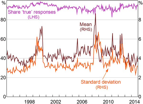
Nevertheless, given that the standard deviation is between 2 and 7 per cent over time, underlying disagreement among consumers is still substantially larger than disagreement among professional forecasters. Previous work has documented a similar pattern internationally (Ranyard et al 2008; Armantier et al 2013).
Compared with the raw data, the estimated underlying level of disagreement is much more stable and does not show a trend incline over the early and mid 2000s (Figure 7). In part, this is due to an increase in the weight on the noise distribution over this period, indicating that a greater fraction of people began expecting extremely high levels of inflation. However, most of the difference is due to extreme responses becoming more extreme. This can be inferred from there being little change over the early 2000s in the standard deviation of inflation expectations after removing the highest and lowest 15 per cent of observations each month, as shown by the trimmed distribution in Figure 7.
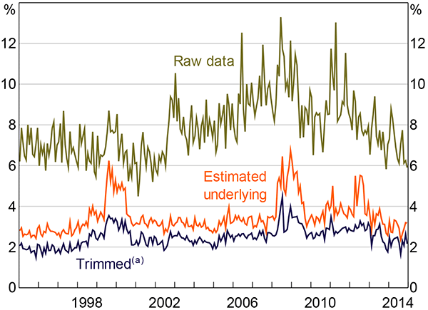
Note: (a) Based on a 30 per cent trimmed distribution
Sources: Authors' calculations; Melbourne Institute of Applied Economic and Social Research
Unlike the professional forecasts, underlying disagreement in consumer inflation expectations exhibits no trend decline over the inflation-targeting period. This could provide less compelling support for increased anchoring; however, this may simply be a result of the short sample of micro data available. In fact, if the positive correlation between the mean and standard deviation seen in Figure 6 (and formally tested in Section 5.2) holds through the history of the sample, disagreement among consumers may have fallen in the early 1990s together with the fall in mean inflation expectations (Figure 8). Unfortunately, micro data prior to 1995 are unavailable to test this possibility.
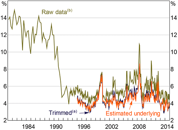
Notes:
(a) Based on a 30 per cent trimmed distribution
(b) A series break occurs prior to January 1995 due to a change in methodology
Sources: Authors' calculations; Melbourne Institute of Applied Economic and Social Research
Footnotes
The correlation between these measures is not primarily due to a common downward trend. For the detrended series, the correlation between the RBA and union survey measures falls to 0.19, but the other pairwise correlations are similar. [3]
The pre-inflation targeting maximum inflation rate was around 25 per cent, during the early 1950s wool boom. [4]
Another possibility is that these extreme values result from data entry errors, which would also act to introduce noise and distort measures of disagreement. [5]
An evaluation of our approach relative to more sophisticated non-parametric methods in the robust statistics literature is beyond the scope of this paper. The validity of the structure we impose depends on the underlying data generating process, which is unknown. [6]
Some fraction of responses equal to a multiple of five may represent ‘precise’ answers. Appendix A outlines a method to estimate this fraction. The estimated parameters of interest are similar using this more complicated method to those using the model outlined here. [7]
We discard twelve observations below −50 per cent and one observation above 100 per cent from the dataset since they are particularly extreme outliers. [8]
The lowest and highest categories are not centred on j, but this has a negligible effect because observations within this range are almost entirely accounted for by the ‘noise’ distribution, as described in what follows. [9]
Observations are weighted by their sampling frequency, as is standard for Melbourne Institute's stratified dataset. [10]


