Bulletin – September 2015 Global Economy Explaining the Slowdown in Global Trade

Introduction

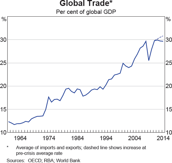
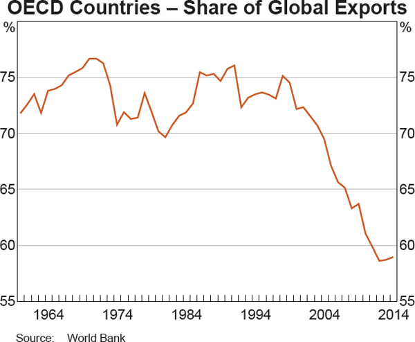
Before the global financial crisis, international trade had been growing at about 1½ times the rate of global GDP for around four decades, resulting in a substantial increase in the global trade-to-GDP ratio (Graph 1). The increase in trade over this period is widely attributed to structural factors, including substantial declines in the cost of trade, expansions of global supply chains and the increased importance of emerging economies in international trade (WTO 2013). Trade as a share of GDP increased dramatically over this period for emerging economies, like those in east Asia. In contrast, trade as a share of GDP in the United States and other advanced economies increased at a slower pace and their share of global merchandise exports has declined since the early 1990s (Graph 2).

Since the financial crisis, however, growth in global trade has not resumed its earlier pace. Growth rebounded strongly in 2010, following widespread recession, but real global trade has subsequently grown at an average annual rate of around 2 per cent, well below the pre-crisis average of 6½ per cent. Sustained weakness in economic growth, especially in advanced economies, can help to explain the slowdown in trade. But over the past four years trade has grown at an even slower rate than GDP, resulting in the ratio of trade to GDP falling a little over this period. This has led to some suggestions that the slowdown in trade might be of a more permanent, or structural, nature.

This article reviews possible structural and cyclical factors behind the recent slowdown in global trade and finds evidence that a large part of the slowdown in trade can be explained by cyclical factors. This suggests that if growth in global business investment, which is the most import-intensive component of demand, were to pick up to pre-crisis levels and the general economic uncertainty were to dissipate, growth in trade would also be likely to increase again.

Structural Explanations for the Slowdown

One possible explanation for the recent slowdown in global trade is that structural policies and factors that had boosted trade, such as trade liberalisation and supply-chain expansion, have largely run their course. In support of this explanation, Ferrantino and Taglioni (2014) note that trade in complex goods typically associated with supply chains has grown particularly slowly after the financial crisis. Constantinescu, Mattoo and Ruta (2015) argue that trade has become less responsive to changes in income since the early 2000s, perhaps because of a slowing in the pace at which supply chains are internationalising.

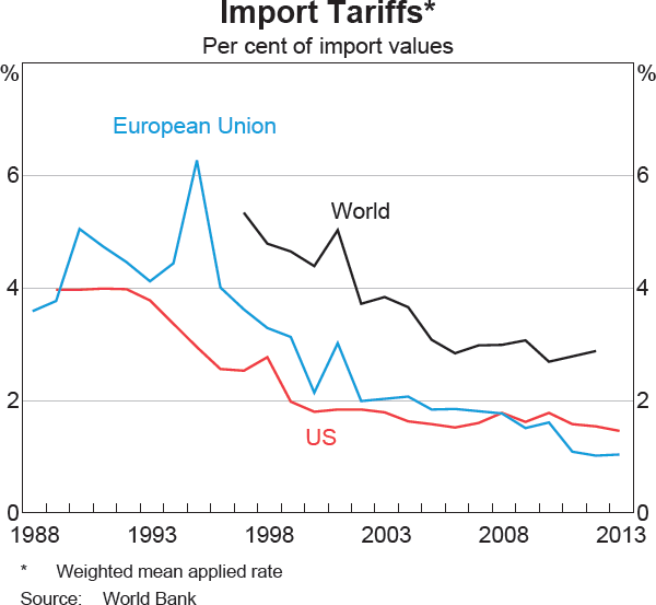
Nevertheless, it may be too early to conclude that structural expansion in trade is over. Global supply chains are still a relatively recent phenomenon and increasing demand for consumer durables from emerging economies is likely to boost the importance of the large-scale, efficient production that they afford. There is also potential for further trade liberalisation. According to the World Trade Organization, the average good imported into the United States or the euro area still faces around a 1½ per cent tariff and the average global import faces a tariff of around 3 per cent (Graph 3). Furthermore, other economically significant non-tariff barriers, such as anti-dumping and ‘buy local’ legislation on government purchases, remain in place in many countries (Evenett 2014).

Cyclical Explanations for the Slowdown

Cyclical factors, such as the composition of the recovery in global GDP growth and lingering economic uncertainty following the crisis, could also help to explain the slowdown in trade growth relative to GDP growth.

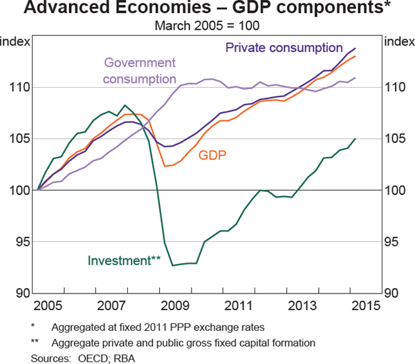
Domestic demand is an important driver of imports in most economies. Business investment is usually the most trade-intensive component of domestic demand because firms often require specialised capital goods not available locally and typically have more direct international access to purchase goods from overseas than do households (see, for example, Bems, Johnson and Yi (2013); Bussière et al (2013)). As a result, the continuing weakness in business investment, relative to other components of demand, is likely to have slowed growth in global trade in the post-crisis period (Graph 4).

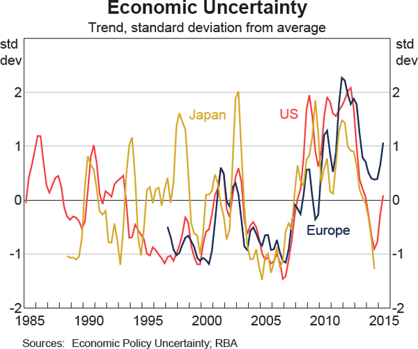
Measures of economic uncertainty have been elevated since the financial crisis, reflecting, in part, difficulties in forecasting the timing and pace of economic recovery, and this may also have weighed on trade (Graph 5). Novy and Taylor (2014) argue that a large part of the collapse in trade during the financial crisis can be attributed to uncertainty. They showed that an increase in uncertainty altered firms' inventory policies, and if firms reduced foreign orders by more than domestic orders, this could lead to a bigger contraction in international trade flows than in domestic economic activity. Uncertainty can also affect trade by restricting credit growth, to which trade appears to be particularly sensitive (Chor and Manova 2012).

Estimating the Contribution of Cyclical Factors to the Slowdown

An econometric model can be used to quantify the contribution of both the weak recovery in the post-crisis period in the components of aggregate demand that have high import intensity and the lingering economic uncertainty during this period. The import demand model of Bussière et al (2013) is augmented with a measure of economic uncertainty from Baker et al (2015) for this purpose.^[1]

Bussière et al's model relates imports to relative prices and a measure of aggregate demand that weights the expenditure components according to their import intensities. This import-adjusted demand measure (IAD), has the form:

where c, g, i and x represent the expenditure components of GDP (private consumption, government consumption, investment and exports, respectively) of country j while ω represents the import intensity of each component.^[2] For example, in 2005, the import content of Australian investment was 26 per cent, a bit higher than that of private consumption at 18 per cent and exports at 14 per cent. The import content of government consumption was relatively low at 10 per cent. Bussière et al find that the import-adjusted demand measure explains the fall in trade volumes during the crisis better than other, more traditional, demand measures, such as domestic demand or GDP.

This article re-estimates Bussière et al's model, updating the sample period to the first quarter of 2015 and adding economic uncertainty as an explanatory variable, and examines its performance during the post-crisis slowdown. Specifically, the following equations for imports are estimated for a panel of 18 advanced economies, using data from the OECD's harmonised national accounts database.^[3] In the models, the quarterly growth of real imports (ΔInm_j,t) depends on the quarterly growth rates of aggregate demand (ΔInD_j,t); relative import prices (ΔInRPM_j,t); uncertainty (ΔInUNC_j,t); and time-invariant country-specific factors (FE_j). IAD, domestic demand and GDP are alternatively used as the measure of aggregate demand (D_j,t).

The econometric results suggest that the relative slowdown in aggregate global trade growth can be largely explained by cyclical factors. The parameters are statistically significant (with one exception) and take their expected signs: higher demand has a positive effect on import growth, while higher import prices and an increase in uncertainty tend to have a negative effect on imports (see Table A1).^[4]

The models using the IAD measure of domestic demand perform noticeably better over the full sample (1985:Q2 – 2015:Q1) than the models using the conventional demand variables. The IAD model that includes a measure of economic uncertainty has the most explanatory power.^[5]

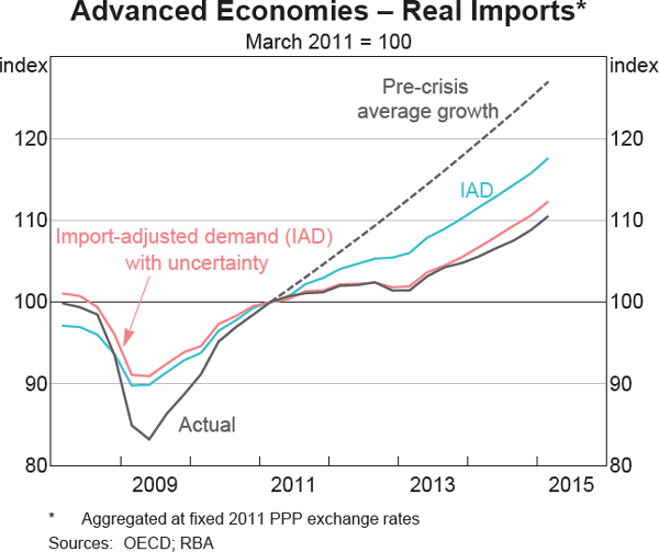
To analyse the performance of these models over the recent period, they are re-estimated using data up to the end of 2010, so that the models ‘observe’ the trade collapse during the financial crisis and the subsequent rebound, but not the recent slowdown in global trade growth relative to GDP growth. The estimated model coefficients are then used to project what the models would have forecast growth to be over the past four years, given the actual movements in the various demand and uncertainty indicators. The resulting projections for the level of import volumes from the IAD model, with and without uncertainty, are shown in Graph 6, along with the actual import volumes. The fitted values from the models prior to 2011 are also shown. Notably, the extent of the decline in trade in 2009 is not entirely explained by the models (although they do much better than the models with traditional domestic demand measures, which are not shown). This is hardly surprising, given the extraordinary circumstances of the financial crisis.

The difference between the dashed line and the blue line on Graph 6 shows that around half of the slowdown in trade growth from its average pre-crisis rate can be explained by the import-adjusted demand model on its own; this result is consistent with other work looking at demand-side factors such as Boz, Bussière and Marsilli (2014) and Morel (2015). Almost all of the remaining slowdown, particularly over the earlier stages of the post-crisis period slowdown, is explained when measures of uncertainty are included in the model.

The IAD model with uncertainty suggests that uncertainty was associated with a reduction in aggregate import growth in both 2011 and 2012 of around 1½ percentage points, and a slightly smaller reduction in the past couple of years. During 2011 and 2012, the uncertainty measures were particularly high, with concerns about a Greek exit from the euro area, debt-ceiling debates in the United States and the upcoming election of the Abe Government in Japan all contributing. Over this period, business investment was particularly weak but, as the blue IAD model line in Graph 6 shows, this alone would not have been enough to cause trade growth to slow as much as it did. As the uncertainty eased and business investment growth picked up in 2013, both models correctly predicted the pick-up in trade. More recently however, through 2014 and early 2015, import growth was slightly slower than the models' prediction.

Although the aggregate slowdown in trade is well explained by the model, the results vary by country. Graph 7 shows the predictions for real imports for selected economies from the IAD model with uncertainty, compared with the actual growth (the solid grey line) and the pre-crisis trend growth (the dashed line) in real imports. The results for the entire sample of countries can be found in Table A2.

For the large euro area economies, such as France and Germany, the model performs fairly well. For Canada, the model under-predicts imports growth slightly, although most of the error occurs in early 2011 and the model-implied growth rates over the rest of the period are broadly in line with the observed data. For the United States, import growth has been below what the model would predict, but demand composition and uncertainty help explain some of the weakness. In Japan, the model under-predicts import growth, which was quite close to its long-run average despite pressure from slowing GDP growth and a substantially lower exchange rate.

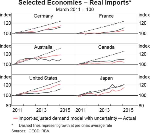
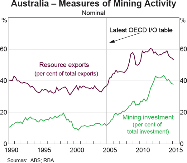
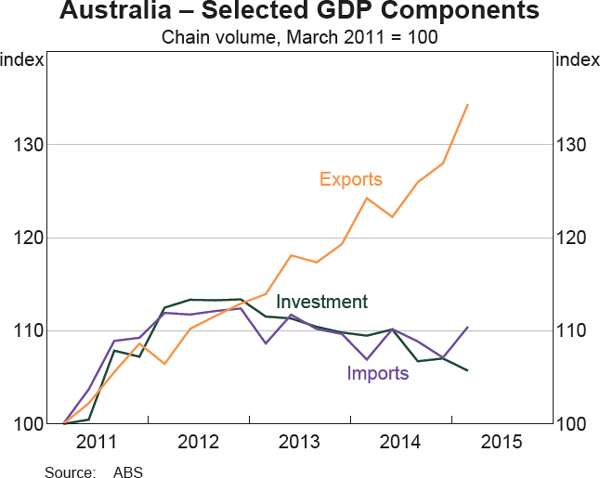
In Australia, the model over-predicts import growth from 2012 onwards. Given Australia's recent resource boom, the 2005 input-output tables by the OECD used to weight domestic demand by import intensity are likely to understate the import content of investment and overstate the import content of exports. This results from mining investment being more import-intensive than other types of investment, and resource exports being significantly less import-intensive than other exports.^[6] Subsequent to the estimation of the 2005 input-output tables, mining investment and resource exports increased substantially (Graph 8). Mining investment peaked in 2012 and has fallen substantially since then, while the volume of resources exports has continued to increase. The model's over-prediction of growth in import volumes since 2012 could therefore be explained by the implicit understatement of the import intensity of resources investment, which is in decline, and overstatement of the import intensity of resources exports, which are increasing (Graph 9).

One potentially important reason for the model fitting the aggregate data better than data on a country level is that the relative import price variables – which measure the national accounts import price deflator relative to the GDP deflator – may not be fully capturing the effects of real exchange rate movements and associated changes in competitiveness. The GDP deflator is a broad measure of domestic prices, which is not necessarily the relevant cost comparison in making decisions about whether to buy domestically or import. These measurement errors are, however, likely to net out in aggregate, but could materially affect country-level results; Morel (2015) finds some tentative evidence for this by comparing the European core to the periphery in a similar model.

Conclusion

Growth in global trade has not recovered to the same extent as global growth in GDP in the period since the financial crisis, perhaps because of a lesser role for structural factors in supporting increased trade of late. However, the relative weakness in global trade growth is well explained by the composition of the recovery in global growth, with investment remaining subdued, and lingering economic uncertainty. This suggests that, should investment recover to pre-crisis growth and the general economic uncertainty dissipate, growth of global trade is likely to strengthen more in line with global GDP growth. Of course, if the slowdown in GDP growth, and investment in particular, are longer-term phenomena, then trade growth is likely to be subdued for an extended period. It should also be noted that this work does not conclusively rule out a moderation in the structural expansion of trade associated with globalisation and industrialisation, but there remain reasons to expect that the structural expansion in trade has further to run.

Appendix A

The baseline regression takes the form:

View MathML

where ΔInm_j,t is the log channge in national accounts imports for country j at time t, ΔlnD_j,t is the log change in the demand measure, UNC_t uses the Baker et al (2013) and Moore (forthcoming) policy uncertainty measures (standard deviations from average level) and ΔInRPM_j,t is the log change in the relative price of imports to domestic goods, measured as the ratio of the import deflator to the GDP deflator. Uncertainty measures are available for the G7 economies and Australia; for others a GDP-weighted average is used as a proxy. The uncertainty measures are not entirely harmonised; for instance, for the United States the measure includes a wider range of factors. Country fixed effects are also included in all specifications (denoted by FE_j).

GDP data are obtained from the OECD harmonised databases; where the harmonised time series are too short, particularly for the relative deflators, the longer series available in the OECD's Economic Outlook database are used. The results are robust to the exclusion of these longer time series in favour of the harmonised data. Data for all countries cover the period 1985:Q2–2015:Q1, except for Germany, which is estimated from 1991:Q1 onwards. For the uncertainty model, the sample period is shorter due to the availability of the uncertainty measures.

Table A1: Estimation Results^(a)

Dependent variable: quarterly growth of real imports, 1985:Q2–2015:Q1

	GDP model	Domestic Demand model	Import-adjusted demand model	Import-adjusted demand with uncertainty
β1	0.48***	0.45***	0.30**	0.21*
Y	1.20***	–	–	–
DD	–	1.38***	–	–
IAD	–	–	1.14***	1.26***
UNC	–	–	–	−0.19***
RPM	−0.15**	−0.04	−0.16**	−0.15*
Observations	2,136	2,136	2,136	1,426
R2(within)	0.16	0.23	0.37	0.47
(a) ***,** and * denote estimates that are significant at 99, 95 and 90 per cent level, respectively. Standard errors are estimated using a clustered sandwich estimator

Table A2: Actual and Predicted Annual Average Real Import Growth

Per cent

	Actual Values			Model Fitted Values in Post-crisis Period(a)
	Pre-crisis (1985–2007)	Post-crisis (2011–2015:Q1)		Import-adjusted demand model	Import-adjusted demand model with uncertainty
Australia	7.2	1.7		4.8	4.7
Belgium	4.9	2.1		2.6	2.7
Canada	5.9	2.5		3.5	1.1
Denmark	4.9	2.5		2.5	1.9
Finland	5.3	0.4		0.1	−2.4
France	5.5	2.2		2.4	1.7
Germany	5.5	2.8		4.6	3.9
Italy	4.7	−2.9		−0.2	−1.0
Japan	4.8	4.6		3.2	3.9
Korea	10.6	2.3		4.7	2.7
Netherlands	5.6	2.3		1.1	0.9
Norway	4.2	1.2		3.2	0.6
New Zealand	5.4	5.9		7.2	5.8
Portugal	7.5	0.8		0.7	−1.4
Spain	9.5	−0.3		2.3	−0.7
Sweden	4.7	2.9		3.6	1.9
United Kingdom	5.5	2.2		3.9	2.1
United States	6.5	2.8		6.3	5.5
Advanced Economies Total(b)	6.1	2.1		3.7	2.4
(a) Using coefficients estimated over the period 1985–2010, fitted to the period 2011:Q1–2015:Q1 (b) Aggregated at fixed 2011 PPP exchange rates

Footnotes

The authors are from Economic Group and International Department. [*]

Where available, the uncertainty measures constructed by Baker et al (2015) (available at <www.policyuncertainty.com>) are used. For European economies without a direct uncertainty measure, the aggregate European measure constructed by Baker et al is used. For non-European countries without uncertainty indices, uncertainty is proxied by a GDP-weighted average of the available uncertainty measures, except for Australia where the measure constructed in Moore (forthcoming, closely following Baker et al (2015)) is used. The country-specific uncertainty measures are relatively highly correlated, so the weighted average is likely to be a reasonable approximation for the countries that have no individual measure available. However, the results are robust to including only those countries for which a direct uncertainty measure is available. [1]

Derived from the OECD input-output (I/O) tables; the weights are time-varying and scaled to sum to one in each period. The I/O tables have three vintages for most countries: 1995, 2000 and 2005. The weights are interpolated linearly between these points. [2]

Only OECD countries are included in the sample, thereby excluding several trade-intensive emerging economies, most notably China. Quarterly national accounts data by component are unavailable for China. Including other emerging Asian economies in the sample was not found to materially affect the results. [3]

Model specifications with lags were also estimated; these were found to improve the fit marginally but did not significantly change the point estimates of the coefficients of interest. Including time-varying fixed effects (assumed to average zero over the sample period) is another way to estimate how cyclical factors affect trade. These parameters are estimated to be negative over most of the post-crisis period, consistent with the results presented below that the trade slowdown is largely cyclical. [4]

Using the post-crisis sample period only, the relative performance of different specifications does not change, and the point estimates for the coefficients are similar. However, the parameter estimates are less precise owing to the shorter sample period. [5]

ABS input-output tables – although not necessarily harmonised to the OECD ones – are available up to the 2009/10 period, which could provide an avenue for future research to test this explanation for the residual. [6]

References

Baker SR, N Bloom and SJ Davis (2015), ‘Measuring Economic Policy Uncertainty’, Economic Policy Uncertainty site. Available at <http://www.policyuncertainty.com/media/BakerBloomDavis.pdf>.

Bems R, RC Johnson and K-M Yi (2013), ‘The Great Trade Collapse’, Annual Review of Economics, 5(1), pp 375–400 .

Boz E, M Bussière and C Marsilli (2014), ‘Recent Slowdown in Global Trade: Cyclical or Structural’, VoxEU site. Available at <http://www.voxeu.org/article/recent-slowdown-global-trade>.

Bussière M, G Callegari, F Ghironi, G Sestieri and N Yamano (2013), ‘Estimating Trade Elasticities: Demand Composition and the Trade Collapse of 2008–2009’, American Economic Journal: Macroeconomics, 5(3), pp 118–151.

Chor D and K Manova (2012), ‘Off the Cliff and Back? Credit Conditions and International Trade during the Global Financial Crisis’, Journal of International Economics, 87(1), pp 117–133.

Constantinescu C, A Mattoo and M Ruta (2015), ‘The Global Trade Slowdown: Cyclical or Structural?’, IMF Working Papers 15/6.

Evenett SJ (2014), ‘The Global Trade Disorder: The 16th GTA Report’, Centre for Economic Policy Research, London.

Ferrantino M and D Taglioni (2014), ‘Global Value Chains in the Current Trade Slowdown’, World Bank – Economic Premise, pp 1–6.

Moore A (forthcoming), ‘Measuring Economic Uncertainty and its Effects’, RBA Research Discussion Paper.

Morel L (2015), ‘Sluggish Exports in Advanced Economies: How Much is Due to Demand?’, Bank of Canada Discussion Paper 2015-3.

Novy D and A Taylor (2014), ‘Trade and Uncertainty’, NBER Working Paper 19941.

WTO (2013), ‘World Trade Report 2013: Factors Shaping the Future of World Trade’, WTO, Geneva.