Bulletin – December 2013 Finance New Measures of Australian Corporate Credit Spreads

Introduction

A number of Australian NFCs are well-established issuers in bond markets, both domestically and offshore. Despite this, historical data on Australian credit spreads are limited, especially at longer maturities.^[1] To address this, the article presents newly constructed measures of secondary market credit spreads for bonds issued by Australian NFCs. Aggregate measures of spreads are estimated as a weighted average of observed spreads of outstanding bonds issued by Australian NFCs, with the weights determined by the distance between the bonds' residual maturities and the target tenor of the estimated spread.^[2] The Bank will publish these measures of credit spreads and yields in a new Statistical Table F3 – Aggregate Measures of Australian Corporate Bond Spreads and Yields.^[3] While the publication of spreads across tenors (3, 5, 7 and 10 years) is subject to the issuance of bonds with such maturities, the method used is relatively robust to changes in issuance trends.

The article proceeds by examining the issuance patterns of Australian NFCs since 2000. This informs the construction of the sample used to estimate the aggregate credit spreads. The estimation method is then discussed. The article concludes by presenting the results obtained for aggregate monthly credit spreads of A-rated and BBB-rated Australian NFCs since 2005.

The Australian Non-financial Corporate Bond Market

Bond issuance by Australian NFCs has grown markedly since the early 2000s.^[4] Over this period, around three-quarters of Australian NFCs' bond issuance has been in offshore markets. Most of the offshore issuance has been denominated in US dollars, reflecting the depth and size of the US bond market (Graph 1). Corporate bond issuers, including Australian NFCs, source much of their longer-term bond funding from the US market where investor demand for longer-dated paper is strong. As a result, the average tenor of offshore issuance has been around 8 years, which is much longer than the typical tenor of slightly above 5 years in the domestic market.

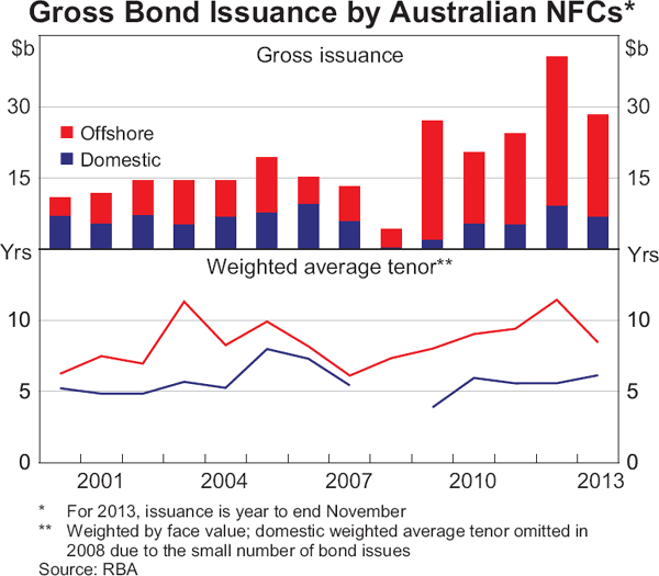
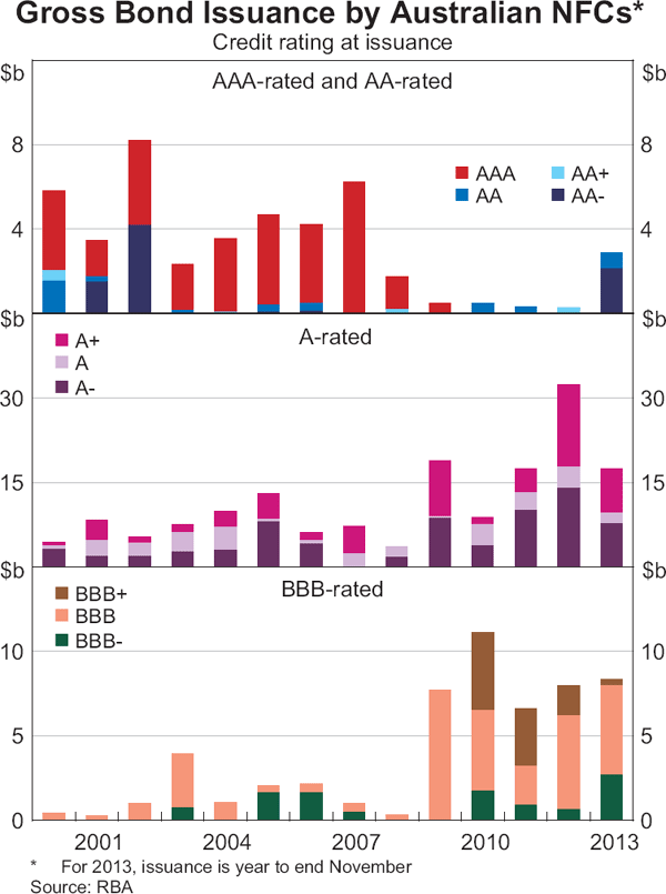
Bond issuance by Australian corporations increased following the onset of the global financial crisis, alongside a decline in equity funding and a global retrenchment in bank loan funding. In recent years, bond funding, and debt funding more generally, have become more attractive for companies because the extended period of low nominal interest rates has seen the cost of debt funding decline to multi-year lows. The majority of issuance by Australian resident NFCs has historically come from companies with a broad A credit rating (A+, A or A−), although issuance by NFCs with a broad BBB credit rating (BBB+, BBB or BBB−) has increased significantly since 2009 (Graph 2). Very few resident Australian NFCs have been rated AA− or higher, resulting in very little issuance at these ratings. Issuance of AAA-rated bonds by Australian NFCs occurred with greater frequency in the years preceding the global financial crisis. These were mainly credit-wrapped bonds – bonds issued by lower-rated entities that achieved significantly higher ratings through insurance provided by specialist bond insurers. These were issued by airports, infrastructure financing vehicles and utility companies. The disappearance of bond insurers following the onset of the global financial crisis has contributed to increased bond issuance at the lower ratings.

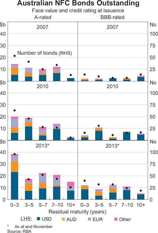
As a result of the historical prominence of offshore issuance, the majority of outstanding Australian NFC bonds are denominated in foreign currencies, particularly in US dollars. By face value, around two-thirds of the bonds currently outstanding are rated A, and this share has increased over time (Graph 3). Close to half of the A-rated bonds are denominated in US dollars, distributed evenly across tenors, while euro-denominated bonds account for around 20 per cent of bonds outstanding. Most of the remaining outstanding A-rated bonds are denominated in Australian dollars, though these tend to be concentrated at the shorter residual maturities (i.e. of less than 5 years). US dollar-denominated securities account for an even larger share of the outstanding BBB-rated bonds. Almost all of the BBB-rated bonds outstanding with residual maturities above 7 years are denominated in US dollars. Australian dollar-denominated BBB-rated bonds are slightly less than 20 per cent of the total outstanding at this rating, and are skewed heavily towards shorter residual maturities. Over time, the value and number of outstanding Australian NFC bonds with longer residual maturities has increased significantly, especially in the 7 to 10 year range.

Sample Construction

The paucity of Australian dollar-denominated issuance by NFCs, particularly at longer tenors, makes it impractical to estimate credit curves across a range of tenors solely from domestically issued bonds. Therefore, the sample includes bonds denominated both in Australian dollars and foreign currencies. An important feature of the longer-term bond issuance by Australian NFCs, and corporate issuers more generally, is the issuance of bonds with embedded options at longer maturities. Reflecting this, the sample includes bullet bonds and bonds with embedded options, such as callable bonds.^[5]

The data in the sample are month-end from January 2000 to November 2013, covering bonds with residual maturities over one year. The sample includes all bonds identified by Bloomberg that were outstanding after 1 January 1990 and were issued by non-financial entities incorporated in Australia.^[6] The sample is restricted to fixed-rate NFC-issued bonds raising the equivalent of at least A$100 million. The sample covers bonds denominated in Australian dollars, US dollars and euros. A total of 555 securities met these criteria, comprising 455 bullet bonds and 100 bonds with embedded options.^[7]

Where a US dollar-denominated bond line had both 144A and Regulation S series, the latter were omitted to avoid duplication, as these are effectively the same bond but issued under different regimes, reducing the sample by 77 securities.^[8] A further seven securities were excluded because of other forms of duplication.^[9] The sample also excludes a number of securities that were downgraded multiple notches by credit ratings agencies during, or shortly after, the onset of the global financial crisis. This meant excluding seven credit-wrapped securities, mostly bonds that were originally AAA-rated and were issued by airports and utility companies prior to 2008, and one bond which was downgraded to sub-investment grade status in early 2009.

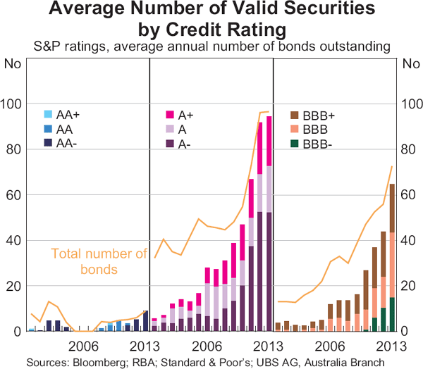
The analysis primarily uses corporate bond price data from Bloomberg's BVAL pricing source, which combines information from a number of sources to generate a ‘best-available’ data point.^[10] These data are supplemented, in order of priority, by Bloomberg generic prices and UBS data.^[11] This approach is guided by an overarching objective to produce transparent credit spread measures derived from price observations provided by multiple contributors. The lack of historical bond price data is the main impediment to producing historical credit spread measures. However, the number of valid observations in the sample – bonds with prices, reported face values and available credit ratings – improves considerably over time as a share of the total number of bonds outstanding in the sample (Graph 4). Prior to 2005, around 25 per cent of the bond sample had adequate pricing data (mainly prices available from UBS). Data availability increases to around 50 per cent of the sample between 2006 and 2009, which largely reflects the availability of Bloomberg's BVAL pricing after 2008, before improving thereafter to over 80 per cent by 2013.

The analysis is conducted directly on corporate bond spreads over corresponding swap rates, which has two advantages: (1) credit spreads to swap can be sourced directly and consistently from Bloomberg; (2) hedging the credit spreads of foreign currency bonds into Australian dollar equivalent spreads, which as explained later is required for comparability within the sample, requires the calculation of swap spreads.

Traditionally, most bonds issued by Australian NFCs have been bullet securities, where the face value of the bond is redeemed at maturity. For these securities, obtaining the spread to swap is straightforward and is calculated as the security's yield to maturity over the corresponding interpolated swap rate. For Australian dollar bonds, this is the spread over the Australian dollar swap curve, which is an interpolated quarterly swap rate for tenors between 1 and 3 years, and a semiannual swap rate for tenors of 4 years and above.^[12]

The analysis is complicated by the inclusion of bonds with embedded options, where the optionality affects the underlying value of the bond and, in turn, its yield and swap spread. This requires the use of an option adjusted spread (OAS), which measures the spread that is not attributable to the value of the option.^[13] The inclusion of securities with embedded options increases the sample of bonds with valid pricing (Graph 5). Because these securities tend to be over-represented at longer maturities, their inclusion assists in producing credit spread measures for longer tenors.

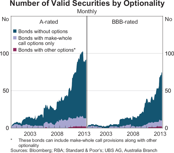
For comparability within the sample, the credit spreads on foreign currency denominated bonds are converted to their Australian dollar equivalent spreads, which corresponds to the foreign exchange risk on the foreign currency bonds being completely hedged (see Appendix A for a discussion of the hedging method). Given the small number of bonds with a credit rating above AA−, only bonds with broad A and BBB credit ratings are included in the analysis. Individual bond ratings issued by Standard & Poor's (S&P) are used where available, and S&P's issuer rating otherwise.

The final sample captures around 90 A-rated securities and around 60 BBB-rated securities on average in 2013, with a significant increase in the sample size over time (Graph 6). The number of unique issuers included in the sample has also increased over time.

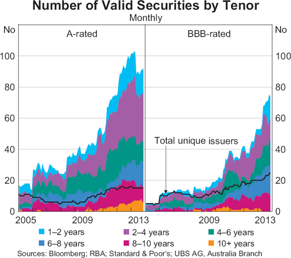
Based on the available data, it is possible to produce aggregate credit spreads from 2005 onwards. The choice of starting point attempts to balance the representativeness of the estimates with a desire to produce a historical time series of reasonable length. However, because of the smaller sample size, estimates generated for the A-rated bonds prior to 2008, and before late 2009 for the BBB-rated bonds, may be less representative of the underlying market than the estimates obtained for more recent years.

Estimating the Australian NFC Credit Spread Curve

Robust estimates of credit spreads for a given rating require the availability of a sufficient number of bonds, distributed widely across tenors. Despite the increase in the number of bonds in the broad A and BBB ratings since the mid 2000s, the number of bonds within the fine credit ratings remains relatively low. As a result, aggregate credit spreads are estimated separately at only the broad A and BBB credit ratings.

A number of methods are available to estimate credit spreads. In this article, aggregate credit spreads of A-rated and BBB-rated Australian NFCs are estimated for a given (target) tenor as the weighted average of the Australian dollar equivalent credit spreads over the swap rate. The method is applied to the cross-section of bonds in the sample that have the desired credit rating. The weights are determined by a Gaussian kernel that assigns a weight to every observation in the cross-section depending on the distance of the observation's residual maturity and the target tenor according to a Gaussian (normal) distribution centred at the target tenor.^[14] This method recognises the fact that the observed spreads on bonds with residual maturities close to the target tenor contain more information about the underlying spread at that tenor than spreads on bonds with residual maturities further away. The advantage of the Gaussian kernel over other more simplistic weighting methods, such as an equally weighted average, is that it uses the entire cross-section of bonds, albeit with weights approaching zero as the distance of the bonds' residual maturity from the target tenor increases. This provides a robust method capable of producing estimates even when the number of available observations is relatively small. The advantage of the Gaussian kernel over parametric methods, that have been popularised in the literature on the estimation of government yield curves, is its simplicity. Also, it does not impose a particular functional form on the credit spread curve but allows the observed data to determine its shape.^[15]

Gaussian kernel weighting

Formally, the Gaussian kernel average credit spread estimator S(T) at target tenor T for a given broad rating and date is:

where w_i (T; σ) is the weight for the target tenor T of the i^th bond in the sub-sample of bonds with the given broad rating, and S_i is the observed spread on the i^th bond in the sub-sample of N bonds with the given broad rating. The parameter σ (sigma), which is measured in years, controls the weight assigned to the spread of each observation based on the distance between that bond's residual maturity and the target tenor (sigma is the standard deviation of the normal distribution used to assign the weights). It determines the effective width of the window of residual maturities used in the estimator, with a larger effective window producing smoother estimates. The general form of the weighting function is:

where K(τ; σ) is the Gaussian kernel function^[16] giving weight to the i ^th bond based on the distance of its residual maturity from the target tenor (|T_t−T|).^[17] F_i is the face value of the i ^th bond, which recognises that larger bond issues are typically more actively traded and are therefore likely to more accurately reflect market conditions.^[18] Finally, the Gaussian kernel is:

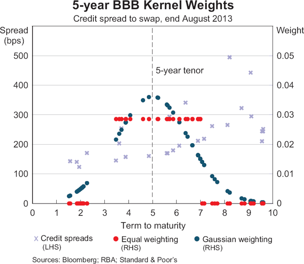
The mechanics of the Gaussian weighting method are illustrated in Graph 7 which shows its application to estimating the 5-year credit spread for BBB-rated Australian NFCs. (For clarity, the illustration abstracts from the impact of the bonds' face values on the weights.) The Gaussian kernel assigns positive weights to all bond spread observations with a BBB rating in the sample's cross-section on the estimation date, but assigns greater weights to the bonds around the 5-year maturity point. This contrasts, for example, with the equally weighted average where observations in the sample are assigned the same weight within some pre-specified range of the residual maturity around the 5-year tenor, but zero weight otherwise.

Optimal smoothing of the Gaussian kernel

The Gaussian kernel method provides a degree of flexibility in weighting the observations around the target tenor through the choice of the value of the smoothing parameter, σ. There is a natural trade-off between the goodness-of-fit of the estimates, measured as the sum of squared residuals between the observed spreads and the estimated spreads, and the smoothness of the resulting credit curve.^[19] Small values of the smoothing parameter produce estimates with smaller residuals by assigning higher weights to bonds closest to the target tenor. However, when the value of the smoothing parameter is too low the estimates are unlikely to be representative of the true credit spread for that tenor, as they reflect more of the noise in the observations. Moreover, the estimates are highly variable (for small changes in the tenor), and can produce credit spread curves that are quite irregular and for which there is little economic justification.^[20] Conversely, higher values of the smoothing parameter produce less variable estimates but may have larger residuals within the sample.

The optimal choice of the smoothing parameter can be made objectively by casting the choice in the same framework as the one for smoothing splines. This involves explicitly trading off the goodness-of-fit of the estimates and the smoothness of the credit spread curve (Anderson and Sleath 2001).^[21] The final choice of the optimal smoothing is also guided by the economic plausibility of the credit spread estimates.

Using the smoothing spline framework, the optimal value of the smoothing parameter on a single date is chosen as the one that minimises the sum of squared residuals of the credit spread estimates, while penalising excessive irregularity (or ‘curvature’) of the estimated credit spread curve:

where S(T_i ; σ) is the Gaussian kernel estimate of the spread at the tenor of the i ^th bond T_i, and S_i is the observed spread of the i ^th bond. The first term of Equation (4) measures the goodness-of-fit of the Gaussian kernel estimate, while the second term measures the curvature of the estimated spread curve.^[22] The parameter λ(0 ≤ λ ≤ 1) controls the trade-off between the fit and the curvature terms in the objective function, with higher values putting more weight on smoothness.

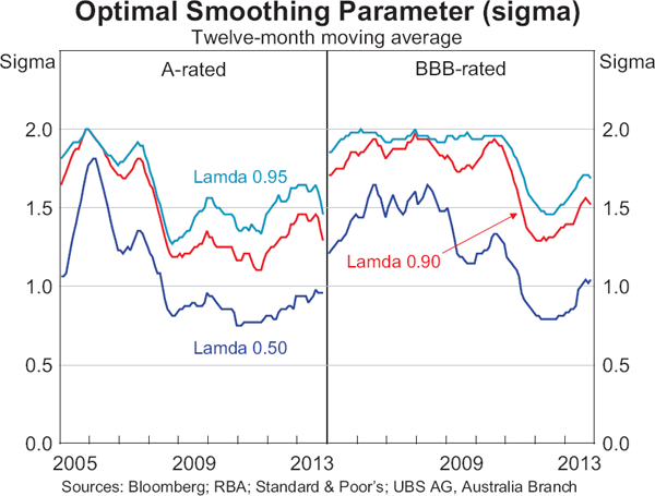
There is little consensus in choosing the trade-off parameter λ.^[23] Considering a range of plausible values for λ showed that for values above 0.9 there is little difference between the optimal sigmas. Relatively low values of λ tend to produce optimal values for the smoothing parameter that appear too small because they result in a large increase in curvature without a significant improvement in the fit. Consequently, the optimal sigma was chosen from the candidates generated by the higher values of λ.

For the A-rated bonds in the sample, a smoothing parameter of 1½ years is optimal and is also relatively stable from 2008 (i.e. the point after which the sample size of the A-rated bonds increases notably; Graph 8). The choice of the optimal value for the smoothing parameter is less clear for the BBB sample, with somewhat higher values for sigma before 2011 but closer to 1½ years thereafter. In the interests of simplicity, credit spreads are estimated with a fixed value of 1½ years for the smoothing parameter throughout the whole estimation period; that is, the weights around each target tenor are determined from a normal distribution with a standard deviation of 1½ years which is centred at the target tenor. This assigns around 50 per cent of the weight to observations with residual maturities within one year of the target tenor, around 80 per cent within two years and around 95 per cent within three years. The choice of 1½ years for the smoothing parameter is further supported by an examination of the credit spreads produced from a range of values for the smoothing parameter (½, 1, 1½ and 2). This revealed that lower values of the smoothing parameter (1 year or less) produce, at times, counterintuitive crossing of the credit spread estimates of different tenors, while higher values of sigma produce what appear to be excessively smooth results.

Australian Non-financial Credit Spread Curves

The credit spreads estimated with the Gaussian kernel are low and quite stable across tenors prior to 2007 (Graph 9). Broadly speaking, the estimated spreads since 2007 have exhibited the expected movements during episodes of financial stress (e.g. during the 2008–09 global financial crisis) and changes in market expectations (e.g. in mid 2013 when financial markets brought forward their expectations for the unwinding of unconventional monetary policies by the US Federal Reserve).^[24]

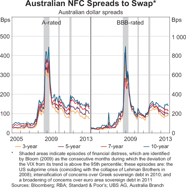
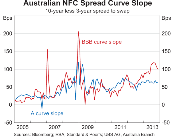
For the most part, since 2005, the credit spread curves of the A-rated and BBB-rated Australian NFCs have tended to shift in parallel across tenors. However, at the height of the global financial crisis in late 2008, when spreads experienced their most significant increase, the credit spread curve steepened sharply, especially for the BBB-rated bonds (Graph 10). Despite the decline in credit spreads since mid 2012, the BBB credit spread curve has steepened by around 50 basis points, suggesting that investors in BBB-rated bonds have, in recent years, required greater compensation for taking credit exposures at longer tenors. Interestingly, this has been accompanied by an increase in issuance of BBB-rated bonds at longer tenors and the downgrade of a number of previously A-rated issuers to the BBB rating.

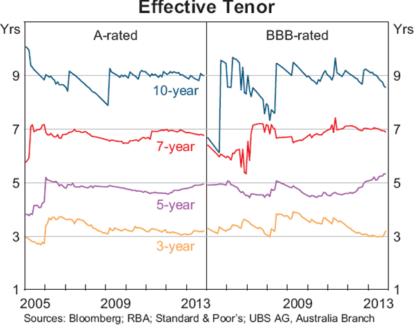
Overall, the Gaussian kernel method produces effective weighted average tenors that are very close to each of the target tenors (Graph 11). The exception is the 10-year tenor where the effective tenor is closer to 9 years. This reflects the dearth of issuance of bonds with tenors of 10 years or more. Notwithstanding the slightly shorter effective tenor for the 10-year point, the estimates of the 10-year spread from the Gaussian kernel are distinct from the estimates of the 9-year spread as the two are estimated by applying different weights to the bonds in the sample.

There are very few alternative measures of Australian credit spreads against which the Gaussian kernel estimates can be compared (Graph 12 and Graph 13).^[25] The Gaussian kernel estimates for A-rated bonds have been consistently below the credit spread series in the Bank's previous Statistical Table F3 since mid 2007 because the latter include (non-bank) financial corporations, such as real estate investment trusts (REITs). These bonds have tended to have higher credit spreads for the same rating than non-financial entities since 2007. The new measures improve the previous series in the Bank's Statistical Table F3 by significantly expanding the sample, separating financial and non-financial corporations, estimating spreads across different maturities, and by using a more robust method that gives greater weight to more representative observations. The new measures of credit spreads for the A-rated and BBB-rated bonds are similar to corresponding measures produced by Bloomberg prior to late 2008. However, they have diverged from the Bloomberg series since then, which reflects in part the counterintuitive behaviour of the Bloomberg spreads between 2009 and 2011.^[26] The new credit spread measures presented herein have a number of advantages. First, the method of the construction is more transparent. Second, the sample is larger due to the inclusion of bonds issued in foreign currencies. Third, the method used is relatively robust, allowing for the estimation of spreads at longer maturities than are available elsewhere.

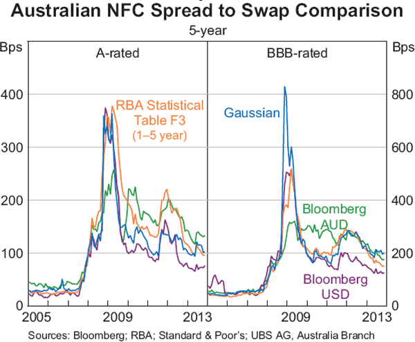
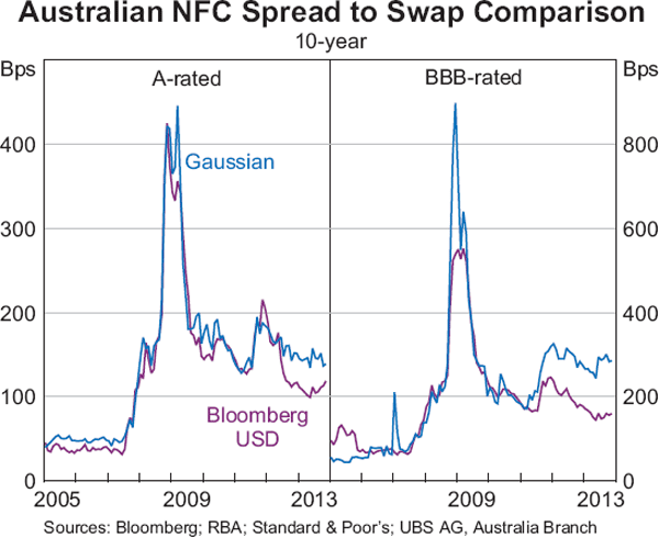
The Gaussian kernel estimates generally track the movement of spreads in global credit markets, in terms of both the timing and severity of their reaction to episodes of financial stress. The levels of the Gaussian kernel estimates of Australian NFC spreads have diverged from their US equivalents since mid 2011, with US credit spreads declining even further than Australian NFC spreads since then. Despite this divergence in levels, the co-movement between Australian NFC spreads estimated with the Gaussian kernel and the corresponding US spreads has remained high.

Conclusion

This article presents a method for estimating aggregate credit spreads across tenors ranging up to 10 years for Australian NFCs. The estimation method is simple, transparent and robust in small samples. The Bank will commence publishing monthly credit spreads estimates from December 2013. The newly constructed credit spread measures will provide richer information than is currently available publicly, allowing the public – researchers, investors, regulators and others – to examine developments in the Australian credit market in more detail.

Appendix A: Hedging Foreign Currency Bond Spreads

To provide comparability within the sample between bonds denominated in different currencies, the analysis converts spreads of foreign currency bonds into their Australian dollar equivalent. This is consistent with corporate bond investors taking a view on credit and interest rate risk only and fully hedging the foreign exchange risk associated with holding foreign currency bonds using derivatives. Moreover, constructing estimates that assume all borrowers hedge in a consistent way allows the analysis to abstract from differences in the methods of hedging (including the use of natural hedges) and the extent of the coverage of hedging. The conversion to Australian dollar equivalent spreads relies on the existence of a well-functioning cross-currency swap market, which is the case for Australia.

Estimating the cost of hedging

Estimating the cost of hedging foreign-issued bonds into their Australian dollar equivalent spread involves a number of stages. This process is only intended as an approximation of the material costs involved. Briefly, these are:

• Cross-currency basis swap: used to convert foreign currency payments into Australian dollars. This is generally the most significant hedging cost.
• Interest rate swap: a basis swap is used to hedge between semiannual coupon payments and the 3-month foreign currency interbank rate, which is typically used as the benchmark for cross-currency basis swap contracts. A basis swap is also used to convert the resulting 3-month Australian dollar equivalent spread to a 6-month equivalent spread for comparability with the semiannual coupons on Australian dollar bonds.
• Conversion factor: adjusts for interest rate differentials when calculating the spread between benchmarks denominated in different currencies. The conversion factor is the ratio of price sensitivities, which translates the relative value of a one basis point change in the interest rate of one currency into the change in another.^[27]

The impact of hedging foreign currency bonds

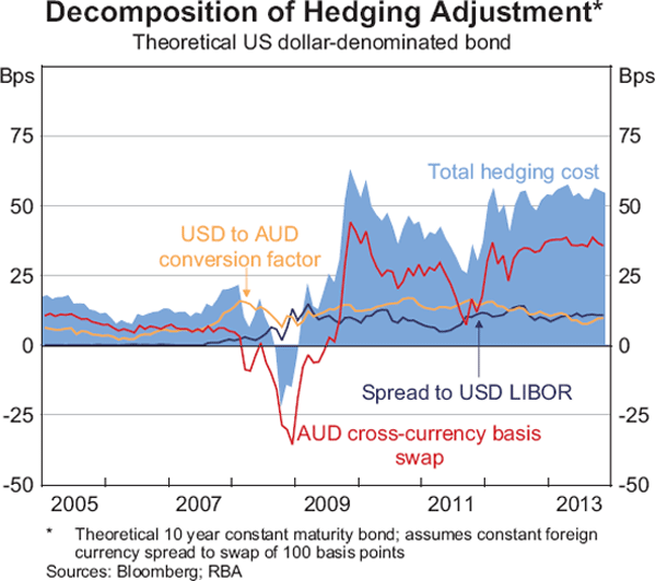
The Australian dollar cross-currency basis swap accounts for most of the foreign currency hedging cost. However, since 2008 the cost of receiving a 3-month foreign currency interbank rate in exchange for a 6-month interbank rate has become a larger component of total hedging costs. To illustrate the evolution of hedging costs, a hypothetical 10-year constant maturity foreign currency bond trading at a foreign currency swap spread of 100 basis points, is hedged from both US dollars and euros. The total hedging cost has been relatively stable since 2010 at around 50 basis points for a theoretical US dollar-denominated bond (Graph A1) and 70 basis points for a euro-denominated bond (not shown).^[28]

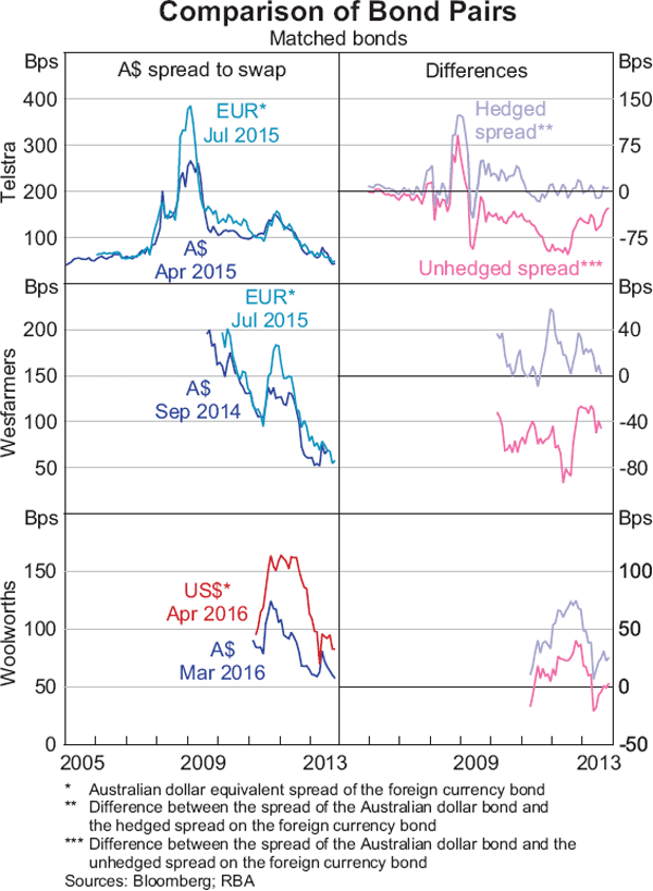
Comparing a selection of bonds also indicates that hedging foreign currency bonds into their Australian dollar equivalent tends to align the spreads more closely with those of comparable Australian dollar bonds. There are only a few instances of comparable pairs of (matched) bonds from the same borrower: bonds with similar residual maturities and issued in a foreign currency and Australian dollars. Despite the small number of bonds in the sample available for comparison, the available observations suggest that the difference between the Australian dollar bond spreads and the hedged foreign currency spreads on comparable bonds tends to be smaller than the difference if the foreign currency bond was unhedged (Graph A2).

Footnotes

The authors are from Domestic Markets Department. Thomas Williams also contributed to the preliminary analysis while he was in Domestic Markets Department. [*]

Besides the difficulty in constructing comprehensive samples of bond data from a range of sources, another factor explaining the lack of such measures is the cost of sourcing, storing and analysing the data for individual bonds necessary to produce measures of aggregate credit spreads. [1]

For a given point in time, the bond's residual maturity measures the time left until its maturity date. [2]

The new table will replace the existing Statistical Table F3 from December 2013. [3]

See Black et al (2012) for a history of Australian corporate bonds. [4]

Bullet bonds are redeemable only at maturity, while bonds with embedded options may have significantly different maturities or cashflows, and as a result different prices and yields, if the embedded options are exercised. Therefore, the latter require the use of option-adjusted spreads to account for the value of their optionality. [5]

Non-financial corporations are identified based on their classification by Bloomberg in a group other than banking, commercial finance, consumer finance, financial services, life insurance, property and casualty insurance, real estate, government agencies, government development banks, governments regional or local, sovereigns, supranationals and winding-up agencies. [6]

The bonds with embedded options include callable, convertible and puttable bonds. [7]

Issuers raising bond funding in US dollars can issue two types of securities for the same bond line that are intended for different investors and classified as either 144A or Regulation S (Reg S). Securities issued under the US Securities and Exchange Commission's Rule 144A are privately placed into the US market and are sold to Qualified Institutional Buyers. Reg S securities are issued in the Eurobond market for international investors and are exempt from registration under the US Securities Act 1933. Each security type is typically assigned its own International Securities Identification Number. [8]

These include duplicate securities available to accredited investors, bonds with warrants and a second series of a bond line. [9]

BVAL pricing is Bloomberg's best-available data point for a given instrument at a point in time. The BVAL price methodology uses three layers of price information, applied in the following order: (1) directly observed data based on traded market prices is used where available; (2) where insufficient data are available, BVAL applies its proprietary correlation model to derive a price from comparable bonds; (3) a relative value yield curve or pricing matrix may be used to derive a price where the correlation model is unable to generate an estimate. A small number of negative bond spread observations were excluded from the sample. [10]

UBS data have previously been used by the Bank to generate the corporate bond spreads and yields series in Statistical Table F3, but are only available for Australian dollar-denominated bullet bonds. For the new dataset presented in this article, UBS data are used only to generate historical estimates before 2009. [11]

While not used in this article, the new measures of credit spreads reported in Statistical Table F3 – Aggregate Measures of Australian Corporate Bond Spreads and Yields, include the credit spread to Commonwealth Government securities (CGS) rates. These are calculated by adding to the estimated credit spread to swap at each tenor the corresponding swap to CGS spread. [12]

Conceptually, the OAS is the constant spread that has to be added to the spot yield curve in an interest rate option pricing model to equate the present value of a bond's cash flows with its market price. The option pricing model needs to make assumptions, including about interest rate volatility. Many bonds in the sample include optionality in the form of make-whole calls. However, the theoretical value of make-whole call options is small (Powers and Tsyplakov 2008) and is not currently incorporated into Bloomberg's OAS spread calculation. As a result, the spreads on bonds with only a make-whole call option are the simple spreads rather than the OAS. Bloomberg's estimates of the OAS are used for the bonds with all other forms of optionality. [13]

For a discussion of the Gaussian kernel and kernel methods more generally, see Li and Racine (2007). [14]

A number of estimation methods were investigated, although the details are not reported here. These methods produced very similar estimates of credit spreads across tenors and broad credit ratings. These methods included a range of parametric models estimated by least squares regressions applied to the cross-section in each period. In particular, the Nelson and Siegel (1987) method was examined in detail owing to its wide use in practice for estimating government yield curves (BIS 2005); this method has also been adapted for the estimation of corporate bond yield and spread curves (Xiao 2010). However, in our sample these models displayed spurious statistical properties, producing very high model fit but largely statistically insignificant coefficients. Other studies have also found evidence of possible over-fitting of the data using parametric methods, particularly in the case of the Nelson and Siegel model (Annaert et al 2013). [15]

A kernel function is a symmetric, continuous and bounded real-valued function that integrates to 1. When the function is constrained to be non-negative it corresponds to a continuous distribution function. There are a large number of candidate kernels, with the Gaussian being the most widely used. Linton et al (2001) examines the application of kernel-based methods to the estimation of yield curves and establishes statistical properties of these estimators. Investigation of a number of other kernel specifications showed that the particular choice of kernel had little material impact on the credit spread estimates. [16]

At the end points of the tenor range (1 and 10 years, but particularly at the 1-year tenor), the Gaussian kernel, and other similar methods, may be somewhat biased because there are no observations below and above the target tenor. Effectively, the weighted average is calculated from bonds on only one side of the estimation window. At the 10-year tenor, this is also an issue due to the sparse issuance above 10 years, but is less problematic for the A-rated bonds, for which some observations are available. However, the degree of bias depends on the true shape of the credit spread curve, with steeper curves resulting in more biased estimates. [17]

The results produced by the Gaussian kernel are very similar when the face values of the bonds are not used in the weighting function; that is, when the weights are based only on the distance between the residual maturities in the sample and the target tenor. [18]

This problem is not unique to credit spreads estimation. Indeed, it is an important consideration in the estimation of government yield curves, where the smoothness of the curve has a direct impact on the quality of the estimated forward rates, which are often used to provide an indication of market expectations of future monetary policy. [19]

The slope at each point of the credit curve for a single issuer can be interpreted as an indicator of the instantaneous probability of default at that point. There are no intuitive or theoretical reasons to expect that the slope of the credit curve, and hence the probability of default, should change significantly for a small change in the tenor. Although this argument only applies to the credit spread curve of a single entity, it is nonetheless a desirable feature of an aggregate measure of credit spreads for a given credit rating. In other words, a priori it would seem reasonable for the slope of the credit curve to change gradually. [20]

A number of risk-free yield curve estimation models use smoothing splines. For examples and details on this approach, see Anderson and Sleath (2001) and Yallup (2012). [21]

In practice, the second derivative in the curvature term is measured by the second difference calculated over a fine grid of tenors. [22]

A popular choice in the risk-free yield curve literature is to set λ by minimising the generalised cross-validation (see Yallup (2012) for an overview). However, even in this setting a choice still needs to be made about the penalty that is applied to the number of model parameters and there is little consensus on this choice. Therefore, the generalised cross-validation approach was not pursued in the analysis. [23]

The episodes of financial market stress are identified from the deviation of the option-implied volatility of the S&P 500 index (VIX) from its trailing average (Bloom 2009). It is not possible to determine with certainty whether the dramatic increase in BBB spreads in late 2008, particularly at the shorter tenors, is overstated owing to the small sample size around this time. During this period, the sample is heavily influenced by the sharp widening of the bond spreads for a major diversified mining company, having considerable influence on the spread estimates around the 5-year tenor. [24]

The available alternative measures are the 1–5 year credit spreads previously published by the RBA in Statistical Table F3 and Bloomberg's proprietary fair value curves. Currently, Bloomberg's fair value curve indices for Australian A-rated and BBB-rated corporate bonds are available up to a maximum tenor of 7 years, with historical data starting in the early 2000s; the Bloomberg indices are produced using a method which is not disclosed publicly in detail. [25]

The Bloomberg Australian dollar fair value curve appears to be overly smooth between early 2009 and late 2010. These measures did not increase as much as could be expected in early 2009, given that the global financial crisis was at its most severe at that time, and as was observed in other measures of Australian and foreign corporate bond spreads. Moreover, the Bloomberg spread measures remained elevated for an extended period of time between early 2009 and 2010, while credit spreads globally declined sharply following the introduction of extraordinary policy measures; this was especially true of BBB-rated bond spreads. [26]

The conversion factor is approximated by the ratio of changes in present value from a one basis point shift in the swap curve at a given tenor for each currency. This approximation, also known as the PV01 (the present value of a one basis point shift in the swap curve), is commonly used by market participants in practice. [27]

The analysis assumes that hedging a euro-denominated bond into Australian dollars first requires euro-denominated cash flows to be converted into US dollar cash flows (incorporating the three factors outlined above), from which Australian dollar equivalent spreads can be estimated. The additional stage reflects the fact that cross-currency basis swaps not involving a US dollar leg tend to be illiquid, and market practice is to hedge first into US dollar cash flows. [28]

References

Anderson N and J Sleath (2001), ‘New Estimates of the UK Real and Nominal Yield Curves’, Bank of England Working Paper No 126.

Annaert J, AGP Claes, MJK De Ceuster and H Zhang (2013), ‘Estimating the Spot Rate Curve Using the Nelson-Siegel Model: A Ridge Regression Approach’, International Review of Economics and Finance, 27, pp 482–496.

BIS (Bank for International Settlements) (2005), ‘Zero-coupon Yield Curves: Technical Documentation’, BIS Papers No 25.

Black S, J Kirkwood, A Rai and T Williams (2012), ‘A History of Australian Corporate Bonds’, RBA Research Discussion Paper 2012-09.

Bloom N (2009), ‘The Impact of Uncertainty Shocks’, Econometrica, 77(3), pp 623–685.

Li Q and JS Racine (2007), Nonparametric Econometrics: Theory and Practice, Princeton University Press, Princeton.

Linton O, E Mammen, J Nielsen and C Tanggard (2001), ‘Yield Curve Estimation by Kernel Smoothing Methods’, Journal of Econometrics, 105, pp 185–223.

Nelson CR and AF Siegel (1987), ‘Parsimonious Modeling of Yield Curves’, The Journal of Business, 60(4), pp 473–489.

Powers E and S Tsyplakov (2008), ‘What is the Cost of Financial Flexibility? Theory and Evidence for Make-whole Call Provisions’, Financial Management, 37(3), pp 485–512.

Xiao J (2010), ‘Term Structure Estimation for U.S. Corporate Bond Yields’, RiskMetrics Journal, 2(1), pp 19–34.

Yallup PJ (2012), ‘Models of the Yield Curve and the Curvature of the Implied Forward Rate Function’, Journal of Banking and Finance, 36(1), pp 121–135.