Research Discussion Paper – RDP 2023-09 Does Monetary Policy Affect Non-mining Business Investment in Australia? Evidence from BLADE
1. Introduction
Non-mining business investment in Australia was fairly weak over much of the 2010s, despite declines in interest rates and moderate economic growth (e.g. Debelle 2017; Heads of Treasuries 2017; van der Merwe et al 2018; Hambur and Jenner 2019). While several explanations have been put forward, such as risk aversion and uncertainty, or pessimism about future outcomes (‘animal spirits’), one potential explanation is that monetary policy is not very effective at stimulating business investment, or has become less effective over time. For example, survey evidence (generally for larger firms) suggests that the hurdle rates that businesses require investments to meet can be ‘sticky’ and not responsive to monetary policy (Lane and Rosewall 2015; Edwards and Lane 2021; Sharpe and Suarez 2013).
As business investment is a key driver of economic growth – both in a structural sense through its contribution to productivity, and in a cyclical sense – it is important to understand how and whether monetary policy affects business investment. The key theoretical channels are well documented. A reduction of the policy interest rate stimulates investment by: increasing aggregate demand; lowering the cost of investment (e.g. borrowing rates) – the ‘user cost of capital’; and loosening credit and financing constraints by freeing up cash flow for indebted firms or raising the value of collateral that firms can pledge to obtain loans (Bernanke and Gertler 1995). However, in practice several factors make it difficult to quantify the effect of monetary policy on investment, and to understand the transmission channels.
A key factor that makes it hard to assess the effect of monetary policy on investment is endogeneity. Softness in (current or expected) economic conditions is likely to lead to expansionary monetary policy, but also to weaker investment, biasing downwards any estimated effect of an interest rate change on investment. Indeed, a negative relationship between investment and interest rates is hard to find in aggregate time series data (e.g. Chirinko 1993; Caballero 1999; Hassett and Hubbard 2002; Cockerell and Pennings 2007). Another factor is that investment is very heterogenous. At any point in time, some businesses are investing a lot while others are not investing, reflecting business-specific conditions and past investment. This can make it hard to identify the effect of monetary policy on investment using aggregate data.
To improve our understanding of the effects of monetary policy on investment we combine the exogenous monetary policy shock measures of Beckers (2020) with quarterly firm-level tax data on the near universe of firms from ABS Business Longitudinal Analysis Data Environment (BLADE). In using firm-level data, we follow earlier work by Ottonello and Winberry (2020), Durante, Ferrando and Vermeulen (2022), Jeenas (2023) and Cloyne et al (forthcoming) in estimating the dynamic effect on investment for a period of up to 12 quarters after a monetary policy shock using a local projections model.
By using firm-level data we can also explore monetary policy transmission channels and whether monetary policy affects different types of firms differently. As well as providing additional insights into how monetary policy works, our work could yield insights into the reasons behind the low levels of non-mining investment evident throughout the 2010s. For example, Cloyne et al (forthcoming) shows that young firms might be more sensitive to monetary policy if they are more credit constrained and expansionary monetary policy alleviates these constraints. If this is the case, declining firm entry rates over the past two decades, and an associated decline in the share of young firms in the economy, could potentially have made monetary policy less effective in stimulating investment. Alternatively, some have argued that the investment of very large ‘leader’ firms is more responsive to monetary policy due to their established relationships with financial institutions, access to various fundings sources and ability to navigate economic fluctuations. If so, then expansionary monetary policy could entrench existing industry leaders and weaken competitive pressures, causing aggregate investment to be weaker than otherwise (Kroen et al 2021; Liu et al 2022). This could potentially help to explain the apparent decline in competition documented in Hambur (2023), which Hambur and Andrews (2023) link to slower investment, particularly among more productive firms.
Our key findings are that contractionary monetary policy decreases both the likelihood that firms invest (extensive margin), and the extent of investment (intensive margin). The effects are economically significant, though it is difficult to compare them to estimates from macroeconomic models given the implied persistence of the shock differs.
We find that firms of different sizes and ages respond similarly to monetary policy shocks, though the likelihood of investing is slightly more sensitive to monetary policy for smaller firms. This has several implications for policymakers:
- The decrease in the share of young firms in the economy, due to slower firm entry, is unlikely to have lowered the effectiveness of monetary policy (at least not directly).
- Recent US evidence that expansionary monetary policy disproportionately supports leader firms, and so reduces competition, does not appear to apply to Australia, at least in terms of tangible investment.
- Survey evidence that large (and some other) firms have ‘sticky hurdle rates’ should not be taken as evidence that they do not respond to monetary policy. This could reflect the fact that monetary policy can affect investment through channels other than by lowering the marginal cost of capital or potential differences between surveyed and actual behaviour.
We also find some evidence that sectors that are more dependent on external finance, and firms that are financially constrained, are more responsive to monetary policy. This highlights the important role that cash flow and financing constraints play in the transmission of monetary policy.
As well as providing Australia-specific results, our work contributes to the broader literature in several ways. First, we provide results for an advanced small open economy, whereas most of the literature has considered larger economies such as the United States (Jeenas 2023; Cloyne et al forthcoming) and the euro area (Durante et al 2022). This is relevant given in a small open economy like Australia, firms are potentially exposed to a greater range of international shocks and not needed given the global cost of capital may play an important role in their financing decisions, rather than only the domestic costs.
Second, we provide some of the first evidence on the effects of monetary policy on expected investment by combining our shock measures with survey measures on expected investment. We find that monetary policy shocks tend to affect both actual and expected investment with a similar lag, rather than influencing expectations earlier. This suggests that firms' expectations are based on current conditions, rather than being based on a clear view of what monetary policy will do to future outcomes.
The economic implications of this finding depend on whether lower expectations of investment translate into lower actual investment in the future. If so, this could be a mechanism through which the effects of economic shocks are perpetuated. If not, there may be limited real economic implications, but this mechanism could lead to cyclical variation in realisation ratios (the ratio of actual to expected investment), which would have implications for practitioners' ability to use these data for economic forecasting.
Third, our finding that monetary policy affects investment on both the intensive and extensive margin speaks to the ongoing discussion on how endogenous capital accumulation should be modelled in macroeconomic models. For example, many models, including Woodford (2005), model investment using convex adjustment costs, leading to smooth investment. This contrasts with the existing evidence (including in this paper) that investment tends to be lumpy. Sveen and Weinke (2007) model lumpy investment; however, they do so using an exogenous Bernouilli process that implies that monetary policy cannot affect the extensive margin of investment, in contrast to our findings. Rather, our results support the use of fixed adjustment costs in investment, as proposed by Reiter, Sveen and Weinke (2013).
2. Data
2.1 Tax data on investment
Our analysis uses quarterly data on gross investment for the near universe of Australian firms for the period between September 2001 and June 2017 from ABS BLADE.[1] The particular data we use are reported in firms' quarterly Business Activity Statement (BAS), in which they report the value of capital purchases they made in the quarter. Our analysis is restricted to the non-primary non-financial private sector. The primary sector (agriculture and mining) is excluded as we expect that commodity prices, rather than monetary policy, are the key driver of investment in that sector. The finance sector is removed due to conceptual difficulties in measuring investment and output in this sector from tax data. And the public sector (health, education, public administration) is removed as fiscal policy is likely to play a more important role in investment in this sector. We also remove firms with no employees as is standard in the literature, though this has very little effect on the results.
We consider both the intensive (how much firms invest) and extensive (whether they invest) margin of investment. We model the extensive margin as an indicator IDi,t, that takes on the value 1 if firm i invests in time t and 0 otherwise. We model the intensive margin as the log of investment Invi,t.
Table 1 provides a summary of the data. The full sample contains around 34 million observations, of which around 29.6 million are from small firms (below 20 employees), 3.9 million are from medium-sized firms (20–199 employees) and the rest are from large firms (200 or more employees). There are a little over 2 million unique firms in each quarter.
Of the 34 million observations, around 9.6 million have positive investment, while the rest have zero investment. This implies that in any quarter, around 28 per cent of firms are investing. The share is lower amongst small firms, where only around 25 per cent invest in a given quarter, and much higher amongst large firms, where around 78 per cent invest in a given quarter (Table A1). The share of firms investing varies moderately over the business cycle, having been strong in the mid-2000s alongside strong economic activity during the mining boom, but lower over the 2010s as overall investment and economy activity also softened (Figure C5). This provides some initial evidence that the extensive margin may be an important margin of adjustment.
Even conditional on investing, the amount of investment is highly heterogenous. While the average investment, conditional on investing is $170,682, the standard deviation is almost $11 million. This also indicates that investment activity is highly positively skewed, with a small number of very large investment observations.
| Mean | Median | Standard deviation | |
|---|---|---|---|
| Extensive margin – % | |||
| Share of firms investing | 28 | ||
| Intensive margin(a) – $ | |||
| Investment, conditional on investing, real | 170,682 | 7,024 | 10,800,000 |
| No of observations | 33,900,332 | ||
|
Note: (a) Capital expenditure deflated to 2017/18 dollars using investment deflator. Sources: ABS; Authors' calculations. |
|||
2.2 Survey data on expected investment
Data on firms' expected investment is sourced from the ABS survey of New Capital Expenditure (CAPEX). This is a quarterly survey of around 10,000 firms. It is a census of the largest investors, with the rest of the sample being made up of a random stratified sample. For our analysis we do not apply sampling weights. As such, for regressions over the entire sample we will overweight large firms (at least in terms of the number of large firms).
Our CAPEX sample is made up of around 519,000 observations covering from September 2001 to June 2021. Consistent with the relatively larger number of large firms in this sample, in any given quarter around 48 per cent of firms have positive investment (Table 2).
As well as asking firms about their current investment, it asks about their short-term and long-term investment expectations. The horizon of these expectations differs based on the calendar quarter, but the short-term expectations tend to cover investment over the next one to two quarters, while long-term expectations cover investment over a period of two to four quarters, starting in one to two quarters in the future. For example, in December 2022 firms will be asked about their expected investment over the next two quarters (short-term expectation), and their expected investment from September 2023 to June 2024 (the 2023/24 financial year; long-term expectations).[2] As discussed in Cassidy, Doherty and Gill (2012) and Berkelmans and Spence (2013), these forecasts are noisy estimates of actual investment, particularly at longer horizons, with firms tending to systematically underestimate their investment.
| Mean | Median | Standard deviation | |
|---|---|---|---|
| Extensive margin – % | |||
| Share of firms investing | 48 | ||
| Share of firms expecting to invest, short-term expectation | 42 | ||
| Share of firms expecting to invest, long-term expectation | 41 | ||
| Intensive margin(a) – $ | |||
| Investment, conditional on investing, real | 2,828 | 118 | 18,984 |
| Investment, short-term expectation, conditional on investing, real | 5,085 | 202 | 31,987 |
| Investment long-term expectation, conditional on investing, real | 9,146 | 346 | 59,335 |
| No of observations | 519,000 | ||
|
Note: (a) Capital expenditure deflated to 2017/18 dollars using investment deflator. Sources: ABS; Authors' calculations. |
|||
3. Methodology
Our analysis closely follows Durante et al (2022), who analyse the heterogeneous effects of monetary policy shocks on European firms' investment. We employ a local projections approach (Jordà 2005) of the following form to trace out the effect of monetary policy shocks (shockt) over a number of horizons (h = 0,...,12).[3]
where Ii,t is our measure of investment (IDi,t or Invi,t). When focusing on the extensive margin, the model is effectively a linear probability model and can be interpreted as the effect on the share of firms investing, or the probability of investing. When the intensive margin is used, we are considering the percentage change in investment for those firms continuing to invest from the quarter of the shock.
The vector Xt–j is a set of control variables, including one lag of firm-level revenue growth, GDP and CPI growth, as well as industry and firm size and age (specifically an indicator if the firm was above or below five years old).[4] As the shocks are exogenous, controls are not strictly needed, but they help improve the precision of our estimates, particularly the firm-level controls. We cluster the errors for each period, allowing cross-sectional correlation across firms. This is important given the variable of interest is the same across all firms for a given period (Cameron and Miller 2015). We do not allow for serial correlation as this is addressed by the lagged variables.
Our measure of monetary policy shocks is the measure constructed in Beckers (2020), which covers the sample period up to December quarter 2018. This is a Romer and Romer (2004) style shock that measures the shock as a deviation from a Taylor Rule, augmented with measures of financial conditions and financial market participants' expectations.
In particular, Beckers (2020) estimates an augmented Taylor rule that includes forecasts for economic conditions, as well as a number of indicators of financial conditions (e.g. bond spreads, option-implied volatility). The shocks are then constructed as the deviation of the actual policy rate from that implied by the rule. He produces two main measures: a preferred measure that also accounts for market expectations for the policy rate, and another version that does not. We use the preferred measure for our analysis, though the results are almost identical using the other measure.
We choose the Beckers measure as our preferred measure as it has been shown to resolve the so-called price puzzle in Australian data: that contractionary monetary policy is often estimated to lead to higher prices. Other measures, including those constructed from high-frequency changes in bond yields, are also explored below.
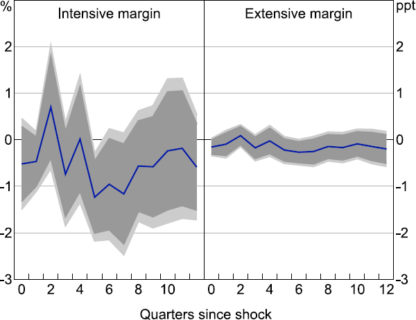
We allow the shock to enter the model directly, similar to Durante et al (2022), rather than using it as an instrument for changes in the cash rate. As such, we are implicitly taking the measure to be a true estimate of the shock, rather than a noisy estimate. That said, the results are reasonably robust to using the shock as an instrument for cash rate changes, which allows for the possibility that the Beckers shock is a noisy proxy for the true shock, though the estimated effects are larger and there is slightly less evidence of significance on the intensive margin (see Figure C6).
4. Results with Tax Data on Actual Investment
Figure 1 shows the results for the full sample. A 100 basis point contractionary monetary policy shock leads to a decline in investment both at the intensive and extensive margin. The decline in both margins is statistically significant (at the 95 per cent level), and peaks after around two years. In terms of magnitude, the share of firms investing falls by a little less than 5 percentage points two to three years after the shock, and the average investment for previously investing firms falls by around 10 per cent.
Interpreting the relative importance of the two channels is difficult, given their different nature. To try to provide some insight we take a simple, back-of-the-envelope approach to quantification. In 2016, the average investment by a firm investing both in the current and previous period (those in the intensive margin estimation) was around $273,000. Taking the peak 10 per cent decline in investment, this equates to $27,300 less per continuing firm. And these firms account for around 17 per cent of the population, so average firm-level investment falls by $4,700. For the extensive margin, average investment for firms investing this period, but not in the previous period, is $52,000. Multiplying this by the peak 5 per cent decline in the probability of investing lowers average firm-level investment by $2,600. So using this simple framework, the intensive margin is about twice as important as the extensive margin.[5]
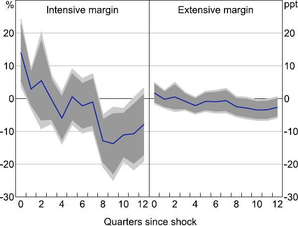
Note: Lighter shaded areas show 95 per cent confidence interval; darker show 90 per cent confidence interval.
Sources: ABS; Authors' calculations.
The timing of the lags with which monetary policy affects investment is consistent with macro models of the Australian economy such as the RBA's MARTIN (Ballantyne et al 2019) and DSGE (Gibbs, Hambur and Nodari 2018) models. However, the response of investment in our results is somewhat larger to that suggested by MARTIN and the DSGE.
One explanation for the larger effects in our results could be the fact that we use nominal measures of investment if tighter monetary policy lowers the price of investment goods. However, when using the aggregate investment deflator we find little evidence that contractionary monetary policy shocks lower the price of investment goods (Figure B3). That said, there is a slight decline in the point estimates, suggesting our estimates of the effect of monetary policy on real investment may be slightly overstated.
Another explanation could be the use of microdata. To consider this, we can estimate the equivalent local projection model using (log) aggregate real non-mining investment (gross fixed capital formation) from the national accounts. We estimate this over a longer sample given the longer sample available (from 1994 to match the shock availability). We again include lagged controls for GDP and CPI growth but have no firm-level controls.
Using the aggregate data, the magnitude and timing of the effects of monetary policy on investment are consistent with aggregate results from the microdata, and are much larger than those from the macroeconomic models (Figure 2). This finding is consistent with Durante et al (2022) and Holm, Paul and Tischbirek (2021) for the euro area and Norway, respectively. It indicates the results are not simply driven by our use of microdata. The finding is robust to changing the number of lags in the controls, adding current controls (to loosen the inherent assumption of no contemporaneous effect from the shock) and accounting for breaks or trends in the level of investment. The results are also similar if we incorporate the Beckers (2020) shocks into a structural VAR with the components of GDP, ordering the shock first, as suggested by Plagborg-Møller and Wolf (2021) (Figure B1).
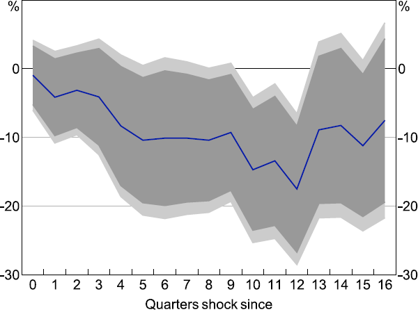
Note: Lighter shaded areas show 95 per cent confidence interval; darker show 90 per cent confidence interval.
Sources: ABS; Authors' calculations.
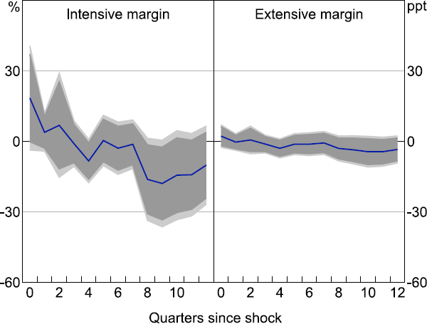
As a final robustness check, we also consider a shock measure derived from high-frequency changes in yields around the time of the RBA's monetary policy announcements (30 minutes before and 90 minutes after) in our microdata regressions. In particular, we use the level shock from Hambur and Haque (2023), which focuses on high-frequency changes in the policy rate.[6] Doing so yields a similar profile for the response of investment to monetary policy, but the size of the response is much smaller and there is less evidence of a significant effect (Figure C7). In part this likely reflects differences in the implicit persistence of these shocks, which can make it hard to compare across shock measures.
More generally, part of the difference between our results and those from existing macroeconomic models likely reflects differences in the implied persistence of the shock. For example, the decline in the cash rate following the shock in Beckers (2020) is much more persistent than that implied by the Taylor rules in MARTIN or the RBA's DSGE model. As such, we may not be comparing like for like. Following an initial shock of 100 basis points, the cumulative change in the cash rate is almost 900 basis points in Beckers (2020) and only around half that in the DSGE, while in MARTIN interest rates very quickly fall and overshoot such that the cumulative change in interest rates over three years is near zero.
Still, taken together the results provide strong evidence that contractionary monetary policy leads to lower investment, though the exact magnitude of the effect is uncertain and can vary depending on the modelling approach and the shock measured used.
4.1 Results by firm size and age
We next explore whether our microdata results differ by firm size or age. This is important for two reasons. First, any difference in results along these dimensions can help us to think about the transmission channels of monetary policy. Small and young firms may tend to be more financially constrained, with lower levels of free cash flow. As such, if these firms' investment decisions are more responsive to monetary policy, this may suggest that monetary policy affects investment by influencing financing constraints.[7] Second, over the past decade there has been a sharp decline in firm entry and exit, meaning that there are fewer young firms in the economy. If young firms' investment is more responsive to monetary policy, this change in firm demographics could weaken the effects of monetary policy and potentially help to explain the subdued levels of non-mining investment evident in the 2010s.
Focusing first on size, Figures 3 and 4 show the results from splitting the sample into small (< 20 staff), medium (20–199 staff) and large firms (200+ staff). Overall, there is some statistical evidence that the extensive margin plays a slightly more important role for small firms, consistent with these firms investing less regularly than larger firms, but aside from this the differences appear small (see Figure C1).
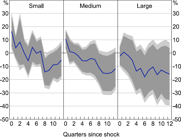
Note: Lighter shaded areas show 95 per cent confidence interval; darker show 90 per cent confidence interval.
Sources: ABS; Authors' calculations.
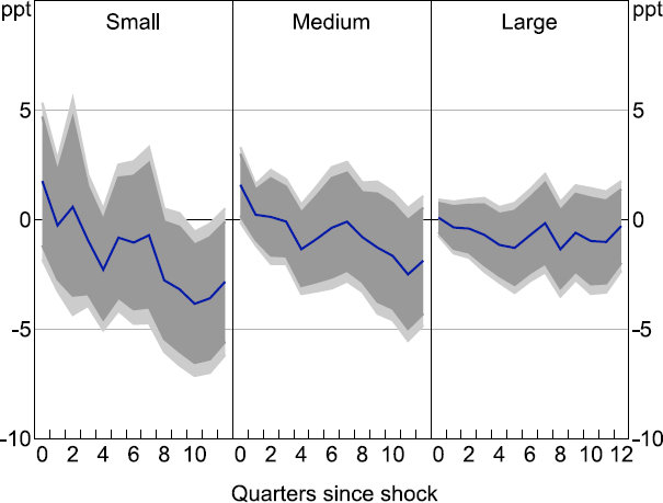
Note: Lighter shaded areas show 95 per cent confidence interval; darker show 90 per cent confidence interval.
Sources: ABS; Authors' calculations.
Considering age, the results are again similar across young (0–5 years) and old (5+ years) firms with no evidence of a significant difference in the effects (see Figures 5 and C2). This suggests that the decrease in the share of young firms in the economy witnessed over the past decade is unlikely to have caused aggregate investment to become less responsive to monetary policy.
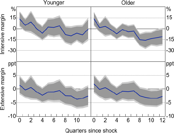
Note: Lighter shaded areas show 95 per cent confidence interval; darker show 90 per cent confidence interval.
Sources: ABS; Authors' calculations.
This finding is somewhat different to Cloyne et al (forthcoming), who find that younger firms in the United States, particularly non-dividend-paying ones, respond more strongly to shocks, reflecting greater financing constraints. One difference is that they focus on listed firms, whereas we focus on a much larger sample of firms; as such, more of the older firms could be financially constrained in our sample. They also focus on a higher age cut-off of 15 years for young firms.[8]
4.2 Results by leader versus non-leader
Another way to think about firm size is to define industry ‘leaders’, the largest 5 per cent of firms in a 4-digit ANZSIC industry, and ‘non-leaders’. This allows us to abstract from inherent differences in firm sizes across industries and to focus on the largest firms in each industry.
We use this split to think about two key aspects of monetary policy pass-through. The first is whether evidence that firms have sticky hurdle rates should be taken as evidence that they do not respond to monetary policy. For example, survey evidence suggests that firms' hurdle rates do not respond to interest rate changes (Lane and Rosewall 2015; Edwards and Lane 2021). Some of these surveys are focused on industry leaders. If leader firms' investment does respond to monetary policy shocks, this would indicate that either monetary policy affects their investment through channels other than by lowering the marginal cost of investment, or that the survey responses and actual behaviour differ somewhat.
The second aspect is whether monetary policy could influence the degree of competition in the economy. In particular, recent work in the United States has found that expansionary monetary policy disproportionately supports investment for leader firms, thus undermining competitive pressures in the economy (Kroen et al 2022; Liu et al 2022). We can test whether this is also the case in Australia.
We define leaders based on sales over the previous year. Overall, leaders' investment is slightly less responsive to monetary policy than that of non-leaders, particularly on the extensive margin. But the differences are not statistically significant and are fairly small (Figure 6). And while the responses of leader firms are not significant, this appears to reflect the much smaller sample size, which leads to larger standard errors, rather than a smaller mean response.[9]
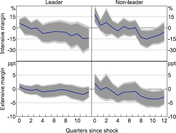
Note: Lighter shaded areas show 95 per cent confidence interval; darker show 90 per cent confidence interval.
Sources: ABS; Authors' calculations.
This finding has two implications. First it suggests that survey evidence that firms', particularly large firms, hurdle rates are sticky should not be taken as evidence that monetary policy does not affect their investment. Monetary policy still affects their investment, though this could be through channels other than lowering their marginal cost of capital. It could also be the case that the surveyed and actual responses differ or that hurdle rates do respond to changing interest rates even if they are sticky. This would be consistent with findings in La Cava (2005) and Hambur and La Cava (2018) that listed companies do change their investment as their cost of finance changes. Our results do not differentiate between these explanations, but they do indicate that evidence of sticky hurdle rates should not be taken as evidence that monetary policy does not affect investment.
The finding also provides some evidence that expansionary monetary policy does not weaken competitive pressures in Australia, as leader firms do not expand their investment by more than other firms following an expansionary shock, in contrast to the US findings. There are several explanations for why our findings differ to the US findings. One is that we use a larger, more representative dataset, which includes more small firms. In contrast, the US work includes only listed firms. This could be important as non-listed firms could be more credit constrained, and so be more responsive to monetary policy.[10]
To consider this, we perform the same exercise, but focus on listed firm data from Morningstar, using the annual dataset outlined in Nguyen (2022). We apply the cleaning method implemented in Kroen et al (2021), removing outliers from the sample. For this analysis we consider both a flow measure of gross investment (as above), and changes in the capital stock (as in Kroen et al (2021)). Unfortunately, the short sample available (from 2001) makes it difficult to draw conclusions around significance.[11] However, focusing on the point estimates there is some tentative evidence that leaders' investment is more responsive to shocks when focusing on larger, listed companies (Figure B2).[12] Taken at face value this could suggest the Kroen et al (2021) result may not hold when considered in a larger, more representative sample, though this would be better tested using comparable US data.
Other potential explanations for the different findings could include the different structure of corporate borrowing in Australia, or the fact that Australia is a small open economy, and so larger firms with access to international capital markets may be relatively more exposed to overseas credit conditions.
4.3 Results by financial dependency
One of the key channels through which monetary policy is thought to affect investment is by influencing financial constraints. This can be through influencing the value of collateral that firms have available to pledge for loans – the so-called financial accelerator channel (Bernanke and Gertler 1995) – or more generally by influencing firms' cash flow and liquidity constraints, or credit supply.
To better understand the financial constraint channel, we explore whether firms that may be more subject to financial constraints, frictions, or are generally more reliant on borrowing, respond differently to other firms following a monetary policy shock. There is a large literature examining the effects of financing frictions and credit availability on firm investment and growth. This literature measures financial frictions and credit supply in numerous ways, and there is no one agreed upon ‘best’ measure of frictions or financial dependence.
For example, Ottonello and Winberry (2020) focuses on leverage and finds that less leveraged firms respond more to monetary policy shocks, which they argue reflects the fact that they have a flatter marginal cost curve. Jeenas (2023) instead focuses on liquidity, and finds that less liquid firms respond more strongly, consistent with monetary policy easing constraints. Finally, Cloyne et al (forthcoming) assume non-dividend-paying young firms are constrained, and find that such firms are more responsive to monetary policy. More generally, thresholds for constraints could differ across firm age, size and industries. And there are difficulties in differentiating between distressed firms, who may be unresponsive, and constrained firms, who may be responsive. As such, we take a different approach.
As our first approach we use industry-level measures of external finance dependence. Specifically we use the measures of US industry-level finance dependence from Demmou, Stefanescu and Arquie (2019), who update Rajan and Zingales’ (1998) approach, and assume these funding structures apply to Australian firms. We split firms based on whether they were in one of the most dependent sectors (top quartile) or least dependent (bottom quartile). Demmou et al (2019) produce these measures on an ISIC Revision 4 basis, and we map them to ANZSIC 4-digit industries.
This measure is constructed using information on the average of the funding requirements of US firms. Using US-based metrics has some advantages and some disadvantages. The obvious disadvantage is that industries may finance themselves differently in Australia and the United States. Still, there are several advantages: using an external dataset limits potential endogeneity concerns; the US data are based on a much longer sample than we have available; the US-based metrics are well-documented and have been used in numerous different studies, making them a robust and comparable set of indicators.
As expected, in sectors that are more dependent on external finance firms' investment appears slightly more responsive to monetary policy shocks (Figure 7). These differences are statistically significant at the 10 per cent level, indicating that more financially dependent sectors are somewhat more responsive, though the magnitude of the difference is not large.[13]
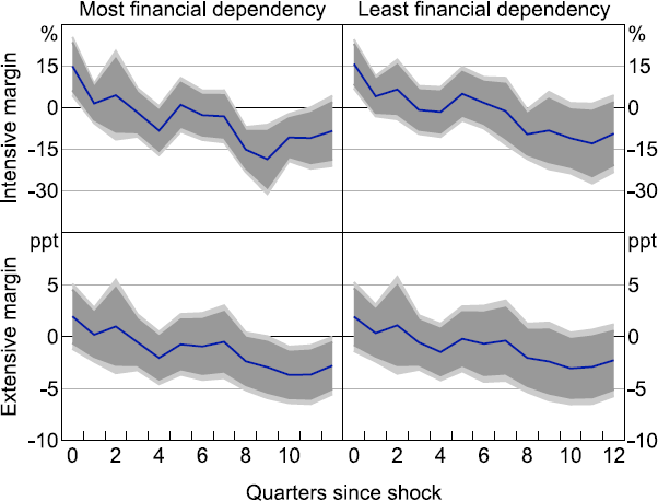
Note: Lighter shaded areas show 95 per cent confidence interval; darker show 90 per cent confidence interval.
Sources: ABS; Authors' calculations.
As a second approach, we take a more direct firm-level financial constraint measure. Rather than base this on balance sheet metrics, we exploit the fact that our data are integrated with survey data from the ABS Business Characteristics Survey, which includes a question asking whether a lack of funds has hampered the firm's operations.[14] While this is only available for a subset of generally slightly larger and older firms, it still provides a large sample for analysis. We also increase the effective size of the sample by classifying firms as constrained if they ever report being constrained in the survey, and unconstrained if they never report being so.[15]
Figure 8 shows the results. The effects for the constrained and unconstrained groups are not significantly different from zero. That said, the effects do appear slightly larger for constrained firms on the extensive margin, and this is borne out in tests of statistical significance, with constrained firms having larger falls in investment at the 10 per cent level (Figure C4). That said, again the differences are not necessarily large economically.
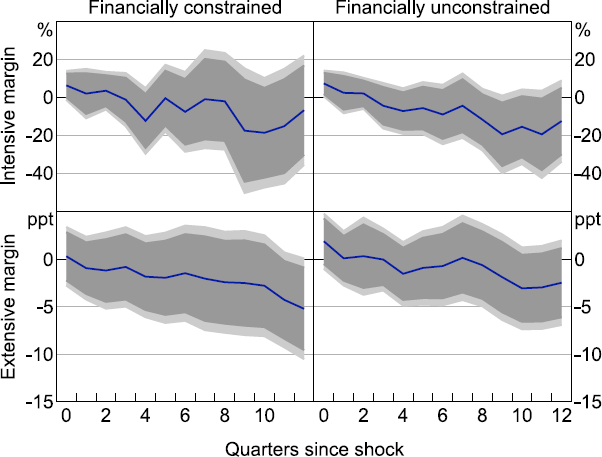
Note: Lighter shaded areas show 95 per cent confidence interval; darker show 90 per cent confidence interval.
Sources: ABS; Authors' calculations.
Overall, we do find some evidence that firms in sectors that are more reliant on external finance have larger investment responses following a monetary policy shock, and that firms that appear financially constrained are more responsive. This is consistent with monetary policy influencing firms' investment in part by influencing financial constraints.
5. Effect on Expectations with Survey Data
We now turn to the expectations data to better understand how monetary policy affects investment expectations. For the regressions, as well as looking at the effect of the shocks on investment at horizon h , we also look at the effect on expected investment take at time h for the future. More precisely we estimate regressions of the following form:
where k represents the period covered by the short- or long-term expectation measure (e.g. the next quarter or full financial year beginning in a quarter's time). In general, if expectations are rational and forward looking they should be based on expected future outcomes. So if contractionary monetary policy today is expected to weaken outcomes in one year's time, we should expect to see expectations of the investment that will be undertaken next year decline immediately, ahead of any response from actual investment. However, this is not the case.
Overall, it appears that monetary policy shocks affect both actual and expected investment. Somewhat surprisingly though, both appear to respond after around one to two years, rather than expectations falling ahead of actual investment. This is evident in the aggregate CAPEX data (Figure 9), as well as with the microdata, where the extensive margin appears to be the more important margin of adjustment (Figure 10). It also seems to be broadly consistent across smaller and larger firms, though there is some tentative evidence that medium and larger firms adjust their expectations ahead of their actual investment (Figure C8). Taken together, these findings suggest that firms' expectations are largely based on current investment and conditions, rather than reflecting future conditions and how interest rates will affect those conditions.
Whether or not this finding has implications for real economic outcomes will depend on whether these lower expectations feed through to lower future investment. If so, this could be a mechanism through which economic shocks are perpetuated, as occurs in various models with backward-looking expectations (e.g. Brassil, Gibbs and Ryan 2023). If not, the implications may mainly relate to the usefulness of these expectations for economic forecasting. The results would suggest that expectations may lag the cycle somewhat, with realisation ratios tending to be higher around the trough of the cycle, and lower towards the peak. This is consistent with the findings in Cassidy et al (2012). Similarly, these findings suggest that expectations-based investment forecasts may be slow to capture the effects of monetary policy.
Overall, these results suggest that the effects of monetary policy on investment are delayed, hard to predict for firms, and that firms are largely responding to current conditions. This combination of outcomes may provide some insights into which channels of pass through are most important. For example, changes in the marginal cost of capital should likely flow through to firms quickly. So if this was the most important channel, firms should quickly realise that certain projects are not profitable and adjust investment expectations accordingly, which is somewhat inconsistent with these findings. In contrast, firms will only experience the weaker demand stemming from contractionary policy after several periods and may only update their expectations then, which would be consistent with these findings. So the demand channel being particularly important would be consistent with these results. How these findings relate to the financial constraint channel is less clear. Changes in collateral values and therefore borrowing capacity should be evident immediately to firms. However, firms may only realise that they will face cash flow constraints once economic activity weakens, which would be consistent with the delayed response of expectations.
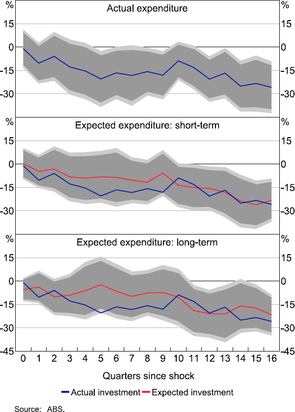
Notes: Non-mining. Lighter shaded areas show 95 per cent confidence interval; darker show 90 per cent confidence interval.
Sources: ABS; Authors' calculations.
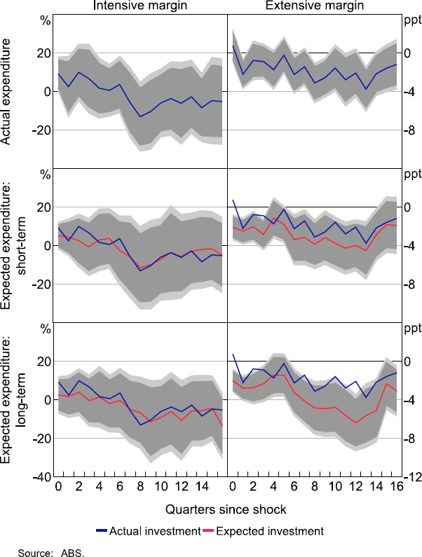
Note: Lighter shaded areas show 95 per cent confidence interval; darker show 90 per cent confidence interval.
Sources: ABS; Authors' calculations.
6. Conclusion
Investment is a crucial driver of economic growth, both in cyclical and structural terms. As such, it is important to understand the extent that monetary policy affects business investment, as well as the channels through which this occurs, as it helps to inform policy, and helps us to understand how the effects of monetary policy could change over time. This is particularly relevant in the context of the surprisingly low levels of non-mining investment evident in Australia over the past decade.
Using exogenous monetary policy shocks and firm-level data we find evidence that monetary policy has a large effect on investment, both on the intensive and extensive margins. We find that contractionary monetary policy decreases both the likelihood that firms invest (extensive margin), and the extent of investment (intensive margin). The effects appear similar across firm age groups, suggesting that the aging of the firm population that has occurred due to declining firm entry rates should not have weakened the effect of monetary policy on investment. The effects are also similar across firm sizes. This suggests evidence that some, particularly larger, firms have sticky hurdle rates should not be taken to indicate that they do not respond to monetary policy.
That said, we do find some tentative evidence that the investment of the largest firms in each industry (‘leaders’) tend to be, if anything, less responsive to monetary policy. This is in contrast to US findings, and suggests that expansionary monetary policy over the past decade is unlikely to have contributed to the weakening in competitive pressures documented in other work (e.g. Hambur 2023).
Moreover, consistent with much of the literature, we find tentative evidence that financial frictions, such as collateral and cash flow constraints, may play an important role in the transmission of monetary policy, given the effect appears larger in sectors that are more exposed to external debt finance and for firms that claim to be constrained. This suggests that monetary policy may be particularly effective in times where these constraints are more binding, such as banking crises or downturns more generally.
Finally, we find evidence that monetary policy also affects investment expectations. However, monetary policy affects actual investment with a lag, and expectations of investment do not anticipate this response. In other words, instead of changing in advance of actual investment as might be expected, expectations move contemporaneously with actual investment. This suggests that reported expectations are somewhat reactive rather than being forward looking, and that forecasts based on these expectations may be slow to capture the effects of policy.
Appendix A: Summary Statistics
| Large | Medium | Small | |
|---|---|---|---|
| BAS(a) | |||
| Share of firms investing – % | 78 | 50 | 25 |
| No of observations | 287,801 | 3,961,966 | 29,650,565 |
| CAPEX(b) | |||
| Share of firms investing – % | 86 | 61 | 24 |
| No of observations | 140,296 | 112,490 | 152,599 |
|
Notes: Size is defined as small (< 20 staff), medium (20–199 staff) and large (200+ staff).
Sources: ABS; Authors' calculations. |
|||
Appendix B: Aggregate Data Results
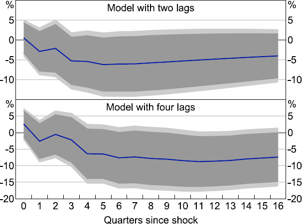
Notes: Small VAR with (log) real trade-weighted index, (log) consumption, (log) non-mining business investment, (log) dwelling investment and cash rate. Lighter shaded areas show 95 per cent confidence interval; darker show 90 per cent confidence interval.
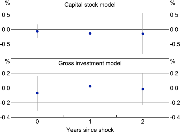
Notes: Model with no growth controls, but with industry*year fixed effects. Dots represent the point estimates of the differences in impulse responses. Bars represent 90 per cent confidence intervals calculated based on a t-distribution with t – n degrees of freedom, where t is number of years and n is the number of coefficients that do not vary across firms.
Sources: Authors' calculations; Morningstar.
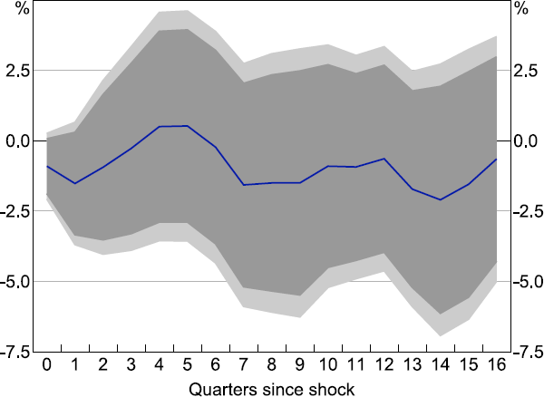
Note: Lighter shaded areas show 95 per cent confidence interval; darker show 90 per cent confidence interval.
Sources: ABS; Authors' calculations.
Appendix C: Additional Microdata Results
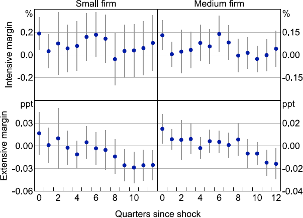
Notes: Dots represent the point estimates of the differences in impulse responses. Bars represent 90 per cent confidence intervals.
Sources: ABS; Authors' calculations.
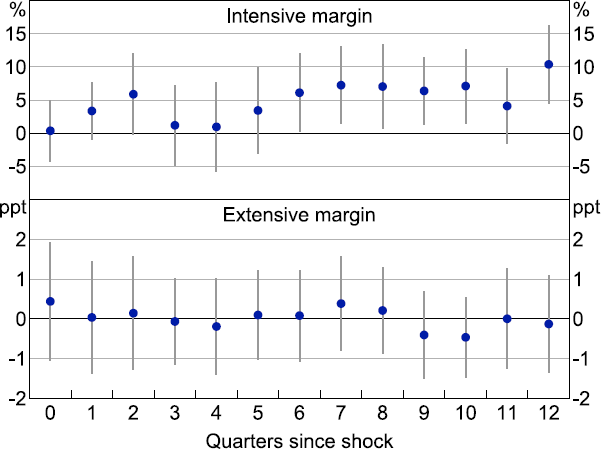
Notes: Dots represent the point estimates of the differences in impulse responses. Bars represent 90 per cent confidence intervals.
Sources: ABS; Authors' calculations.
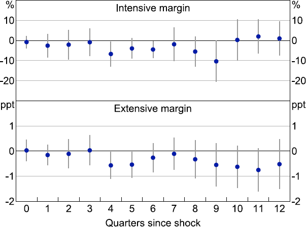
Notes: Dots represent the point estimates of the differences in impulse responses. Bars represent 90 per cent confidence intervals.
Sources: ABS; Authors' calculations.
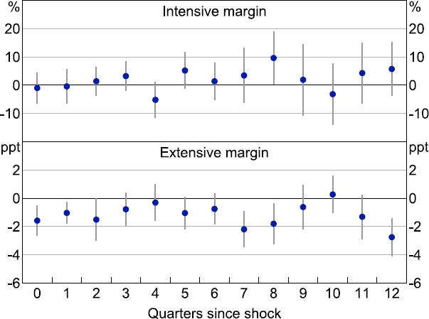
Notes: Dots represent the point estimates of the differences in impulse responses. Bars represent 90 per cent confidence intervals.
Sources: ABS; Authors' calculations.
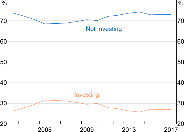
Sources: ABS; Authors' calculations.
Notes: Monetary policy shock is instrumented via cash rate. Lighter shaded areas show 95 per cent confidence interval; darker show 90 per cent confidence interval.
Sources: ABS; Authors' calculations.
Notes: Monetary policy shock is defined as in Hambur and Haque (2023). Lighter shaded areas show 95 per cent confidence interval; darker show 90 per cent confidence interval.
Sources: ABS; Authors' calculations.
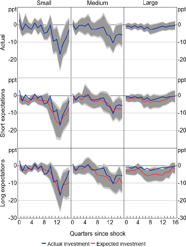
Notes: Non-mining. Lighter shaded areas show 95 per cent confidence interval; darker show 90 per cent confidence interval.
Sources: ABS; Authors' calculations.
References
Ballantyne A, T Cusbert , R Evans, R Guttmann, J Hambur, A Hamilton, E Kendall, R McCririck, G Nodari and D Rees (2019), ‘MARTIN Has Its Place: A Macroeconometric Model of the Australian Economy’, RBA Research Discussion Paper No 2019-07.
Beckers B (2020), ‘Credit Spreads, Monetary Policy and the Price Puzzle’, RBA Research Discussion Paper No 2020-01.
Berkelmans L and G Spence (2013), ‘Realisation Ratios in the Capital Expenditure Survey’, RBA Bulletin, December, pp 1–6.
Bernanke BS and M Gertler (1995), ‘Inside the Black Box: The Credit Channel of Monetary Policy Transmission’, Journal of Economic Perspectives, 9(4), pp 27–48.
Brassil A, CG Gibbs and C Ryan (2023), ‘Optimal Monetary Policy when Expectations are Rational, Fixed, Learned, or Anything in Between’, Unpublished manuscript, Reserve Bank of Australia, 7 September.
Caballero RJ (1999), ‘Aggregate Investment’, in JB Taylor and M Woodford (eds), Handbook of Macroeconomics: Volume 1B, Handbooks in Economics 15, Elsevier Science, Amsterdam, pp 813–862.
Cameron AC and DL Miller (2015), ‘A Practitioner's Guide to Cluster-Robust Inference’, The Journal of Human Resources, 50(2), pp 317–372.
Casiraghi M, T McGregor and D Palazzo (2021), ‘Young Firms and Monetary Policy Transmission’, IMF Working Paper No WP/21/63.
Cassidy N, E Doherty and T Gill (2012), ‘Forecasting Business Investment Using the Capital Expenditure Survey’, RBA Bulletin, September, pp 1–10.
Chirinko RS (1993), ‘Business Fixed Investment Spending: Modeling Strategies, Empirical Results, and Policy Implications’, Journal of Economic Literature, 31(4), pp 1875–1911.
Cloyne J, C Ferreira, M Froemel and P Surico (forthcoming), ‘Monetary Policy, Corporate Finance, and Investment’, Journal of the European Economic Association.
Cockerell L and S Pennings (2007), ‘Private Business Investment in Australia’, RBA Research Discussion Paper No 2007-09.
Debelle G (2017), ‘Business Investment in Australia’, Address to the UBS Australasia Conference 2017, Sydney, 13 November.
Demmou L, I Stefanescu and A Arquie (2019), ‘Productivity Growth and Finance: The Role of Intangible Assets – A Sector Level Analysis’, OECD Economics Department Working Papers No 1547.
Durante E, A Ferrando and P Vermeulen (2022), ‘Monetary Policy, Investment and Firm Heterogeneity’, European Economic Review, 148, Article 104251.
Edwards H and K Lane (2021), ‘Why Are Investment Hurdle Rates So Sticky?’, RBA Bulletin, December.
Gibbs CG, J Hambur and G Nodari (2018), ‘DSGE Reno: Adding a Housing Block to a Small Open Economy Model’, RBA Research Discussion Paper No 2018-04.
Hambur J (2023), ‘Did Labour Market Concentration Lower Wages Growth Pre-COVID?’, RBA Research Discussion Paper No 2023-02.
Hambur J and D Andrews (2023), ‘Doing Less, with Less: Capital Misallocation, Investment and the Productivity Slowdown in Australia’, RBA Research Discussion Paper No 2023-03.
Hambur J and Q Haque (2023), ‘Can We Use High-frequency Yield Data to Better Understand the Effects of Monetary Policy and Its Communication? Yes and No!’, RBA Research Discussion Paper No 2023-04.
Hambur J and K Jenner (2019), ‘Can Structural Change Account for the Low Level of Non-mining Investment?’, RBA Bulletin, June.
Hambur J and G La Cava (2018), ‘Do Interest Rates Affect Business Investment? Evidence from Australian Company-level Data’, RBA Research Discussion Paper No 2018-05.
Hassett KA and RG Hubbard (2002), ‘Tax Policy and Business Investment’, in AJ Auerbach and M Feldstein (eds), Handbook of Public Economics: Volume 3, Handbooks in Economics 4, Elsevier Science, Amsterdam, pp 1293–1343.
Heads of Treasuries (2017), ‘Intergovernmental Review of Business Investment’, September.
Holm MB, P Paul and A Tischbirek (2021), ‘The Transmission of Monetary Policy under the Microscope’, Journal of Political Economy, 129(10), pp 2861–2904.
Jeenas P (2023), ‘Firm Balance Sheet Liquidity, Monetary Policy Shocks, and Investment Dynamics’, Barcelona School of Economics, BSE Working Paper 1409.
Jordà Ò (2005), ‘Estimation and Inference of Impulse Responses by Local Projections’, The American Economic Review, 95(1), pp 161–182.
Kroen T, E Liu, AR Mian and A Sufi (2021), ‘Falling Rates and Rising Superstars’, NBER Working Paper No 29368, rev October 2022.
La Cava G (2005), ‘Financial Constraints, the User Cost of Capital and Corporate Investment in Australia’, RBA Research Discussion Paper No 2005-12.
Lane K and T Rosewall (2015), ‘Firms' Invesment Decisions and Interest Rates’, RBA Bulletin, June, pp 1–7.
Liu E, A Sufi and A Mian (2022), ‘Low Interest Rates, Market Power, and Productivity Growth’, Econometrica, 90(1), pp 193–221.
Morlacco M and D Zeke (2021), ‘Monetary Policy, Customer Capital, and Market Power’, Journal of Monetary Economics, 121, pp 116–134.
Ngyuen K (2022), ‘The Real Effects of Debt Covenants: Evidence from Australia’, RBA Research Discussion Paper No 2022-05.
Ottonello P and T Winberry (2020), ‘Financial Heterogeneity and the Investment Channel of Monetary Policy’, Econometrica, 88(6), pp 2473-2502.
Plagborg-Møller M and CK Wolf (2021), ‘Local Projections and VARs Estimate the Same Impulse Responses’, Econometrica, 89(2), pp 955-980.
Ramey VA (2016), ‘Macroeconomic Shocks and Their Propagation’, in JB Taylor and H Uhlig (eds), Handbook of Macroeconomics: Volume 2A, Handbooks in Economics, Elsevier, Amsterdam, pp 71-162.
Rajan RG and L Zingales (1998), ‘Financial Dependence and Growth’, The American Economic Review, 88(3), pp 559-586.
Reiter M, T Sveen and L Weinke (2013), ‘Lumpy Investment and the Monetary Transmission Mechanism’, Journal of Monetary Economics, 60(7), pp 821-834.
Romer CD and DH Romer (2004), ‘A New Measure of Monetary Shocks: Derivation and Implications’, The American Economic Review, 94(4), pp 1055-1084.
Sharpe S and G Suarez (2013), ‘Do CFOs Think Investment is Sensitive to Interest Rates?’, Board of Governors of the Federal Reserve System, FEDS Notes, 26 September.
Sveen T and L Weinke (2007), ‘Lumpy Investment, Sticky Prices, and the Monetary Transmission Mechanism’, Journal of Monetary Economics, 54(Supplement), pp 23-36.
van der Merwe M, L Cockerell, M Chambers and J Jääskelä (2018), ‘Private Non-mining Investment in Australia’, RBA Bulletin, June.
Woodford M (2005), ‘Firm-specific Capital and the New-Keynesian Phillips Curve’, NBER Working Paper No 11149.
Copyright and Disclaimer Notice
BLADE Disclaimer
The following Disclaimer Notice refers to data and graphs sourced from the Australian Bureau of Statistics' BLADE (Business Longitudinal Analysis Data Environment) database.
The results of these studies are based, in part, on data supplied to the ABS under the Taxation Administration Act 1953, A New Tax System (Australian Business Number) Act 1999, Australian Border Force Act 2015, Social Security (Administration) Act 1999, A New Tax System (Family Assistance) (Administration) Act 1999, Paid Parental Leave Act 2010 and/or the Student Assistance Act 1973. Such data may only be used for the purpose of administering the Census and Statistics Act 1905 or performance of functions of the ABS as set out in section 6 of the Australian Bureau of Statistics Act 1975. No individual information collected under the Census and Statistics Act 1905 is provided back to custodians for administrative or regulatory purposes. Any discussion of data limitations or weaknesses is in the context of using the data for statistical purposes and is not related to the ability of the data to support the Australian Taxation Office, Australian Business Register, Department of Social Services and/or Department of Home Affairs' core operational requirements.
Legislative requirements to ensure privacy and secrecy of these data have been followed. For access to MADIP and/or BLADE data under Section 16A of the ABS Act 1975 or enabled by section 15 of the Census and Statistics (Information Release and Access) Determination 2018, source data are de-identified and so data about specific individuals has not been viewed in conducting this analysis. In accordance with the Census and Statistics Act 1905, results have been treated where necessary to ensure that they are not likely to enable identification of a particular person or organisation.
Acknowledgements
The authors would like to thank Gianni La Cava and Keaton Jenner for sharing their code on earlier analysis of aggregate investment. We would like to thank Gianni La Cava, Elena Durante, Kevin Lane and John Simon for their helpful comments, as well as seminar participants at the RBA, Central Bank of Ireland, and Australian Conference of Economists. The views expressed in this paper are those of the authors and do not necessarily reflect the views of the Reserve Bank of Australia. The authors are solely responsible for any errors.
Footnotes
After 2017 the data collection method changed. For data consistency we end the sample in 2017. [1]
In March 2023 the short-term expectation will be for the next quarter, and long-term is again for the 2023/24 financial year. In June 2023, the short-term expectation is for the next two quarters (September and December 2023), and the long-term expectation is for the subsequent two quarters (March and June 2024). And finally in September 2023, the short-term expectation is for the next quarter (December 2023) and the long-term expectation is for the subsequent two quarters (March and June 2024). [2]
For the analysis using BAS data we only use information out to horizon 12 given the slightly shorter sample. For the rest of the analysis we use data out to horizon 16. [3]
The results are generally robust to including more lags of the right-hand side variables, as well as including the contemporaneous controls which imposes the implicit assumption that monetary policy cannot affect current conditions (Ramey 2016). [4]
This is not surprising given continuing investors account for around 90 per cent of investment. Note that this approach does not take any account of the fact that firms with lower levels of investment may tend to have higher percentage increases, or differences between the marginal firm incentivised to invest by policy and the average firm that moves from non-investing. As such, it should be seen as a very simple indication, not a precise quantification. [5]
This measure is only available for a slightly shorter sample, starting in 2004. [6]
That said, many young firms may not have established banking relationships or may be heavily constrained. This could make them less responsive to monetary policy if policy does not loosen their credit constraints (Casiraghi, McGregor and Palazzo 2021). [7]
While we could explore this higher age cut-off, it is quite high compared to standard definitions of young firms used in administrative data. Moreover, our data has some issues with truncation of ages around the year 2000, with a disproportionate share of firms being born that year. So while we can be confident that for most of the sample (i.e. from around 2005 onwards) firms are at least five years old, the same cannot be said for assessing whether or not they are fifteen years old. [8]
The results are robust to using the current or previous period, and quarterly or annual sales. [9]
Morlacco and Zeke (2021) argue that these dynamics could come through intangible investment, such as investing in branding and customer base. Unfortunately our data are not well suited to test this hypothesis. [10]
We have a very small number of clusters, which can lead to incorrect inference with standard errors. Various approaches have been examined to adjust for small numbers of clusters, but given this regression is not our main focus we do not adopt these. [11]
Results are shown including industry by year fixed effects and removing firm-growth controls to be consistent with Kroen et al (2021). However, the results are very similar if the specification is changed to be similar to our BLADE regressions. [12]
See Figure C3 for test of significance of differences. [13]
The survey covers around 8,000 firms per year. It is a census of firms with more than 300 employees and a stratified random sample for firms with less than 300 employees. Stratification by industry and business size is implemented to produce data that are representative of Australian businesses. The ABS does not provide the sample weights so our analysis is based upon the unweighted data. Firms with fewer than 300 employees are included on a rotating five-year basis. [14]
Splitting firms based on whether they reported being constrained in the previous year provides a similar result. We do not use constrained in the current year as the policy shock itself may influence the firm's constraint status. [15]