Research Discussion Paper – RDP 2023-02 Did Labour Market Concentration Lower Wages Growth Pre-COVID?
1. Introduction
Wages growth was slow in Australia, and many other advanced economies, across a variety of measures in the years leading up to COVID-19 (Australian Treasury 2017; Arsov and Evans 2018). Much of the weakness could be explained by standard determinants. For example, Cassidy (2019) uses one of the RBA's standard models of wages growth to show that most of the decline in wages growth can be explained by higher labour market spare capacity, and lower inflation and inflation expectations. Still, wages growth remained moderately lower than expected even when allowing for these factors. This caused increasing speculation among academics and policymakers about whether deeper structural factors were weighing on wages growth (Lowe 2018; Australian Treasury 2017; Andrews et al 2019; OECD 2020).
The impetus to understand weak wages growth is clear. Wages growth plays a crucial role in inflation dynamics, in determining government revenue, and in the welfare of individuals. Knowing whether and what structural factors are weighing on wages is crucial to understanding future wages growth outcomes. It is also important in creating policy to counter the structural factors. To the extent that these structural factors remain, they could continue to weigh on wages in the post-COVID period.
One explanation that has received attention in recent years is the possibility of decreasing competition and increasing concentration among employers (OECD 2020). All else equal, where there are fewer employers competing for workers, workers have fewer outside options to leverage in wage negotiations. As such, employers tend to have more power to set lower wages. This is referred to as monopsony power.
The focus on employer concentration and labour market power as a potential explanation for low wages growth is unsurprising given the documented increase in concentration in product markets (Hambur forthcoming; De Loecker at al 2020). Increases in employer concentration could help explain other economic phenomena witnessed over the past decade, such as declines in measures of job switching in Australia (Deutscher 2019) and overseas (Moscarini and Postel-Vinay 2017). There is likely to be less job switching when there are fewer employers to switch between.
While numerous papers have documented the impact of employer concentration on wages overseas, there has to date been no work for Australia. Accordingly, in this paper I provide the first Australian evidence using a comprehensive de-identified Linked Employer-Employee Dataset (LEED) based on administrative tax data.
First, I document the degree of concentration in Australian labour markets and how this changed between 2005 and 2016. I find that Australian labour markets are slightly less concentrated than overseas markets, although there is a great deal of variation. For example, more remote markets tend to be more concentrated. Overall, concentration has been broadly unchanged since the mid-2000s.
I then examine the relationship between concentration and wages. I find that wages tend to be lower in more concentrated markets (all else equal), consistent with economic theory. But even within markets there is a lot of variation. Larger firms tend to exert more market power and, therefore, set lower wages (after accounting for differences in productivity). This suggests that models of oligopsony may be more appropriate than models of monopsony, consistent with recent papers such as Berger et al (2021).
Further, the impact of concentration on wages appears to have increased over time. For any given level of concentration, its impact on wages has more than doubled compared to the mid-2000s. So, despite concentration remaining broadly unchanged over the period, it may still have weighed on wages growth pre-COVID. Simple back-of-the-envelope partial equilibrium estimates suggest wages were a little under 1 per cent lower on average from 2011 to 2015 than they would have been had the impact of concentration not increased.
Finally, I examine several potential explanations for the increased impact of given levels of concentration. The results suggest declining firm dynamism and entry rates over the 2010s played an important role as incumbents faced less competition from new firms for workers. In turn, this potentially weighed on aggregate wages growth.
Declines in union membership may have also contributed to the increased impact of concentration by weakening offsetting worker bargaining power as higher levels of union membership appear to provide some offset to employer concentration. However, declining firm entry rates appear to have played a more significant role in making employer concentration more impactful.
Finally, evidence suggests that declining occupational mobility may also have weighed on worker wages by limiting their ability to leverage job opportunities outside their current occupation. However, the interaction between declining occupational mobility and the impact of concentration on wages is less clear.
These results highlight the dual channels through which declining firm dynamism and competitive pressures can weigh on wages growth: indirectly through its impact on productivity (Andrews and Hansell 2021; Andrews et al 2022; Hambur forthcoming); and more directly by impacting worker bargaining power. These results motivate an ongoing focus on potential obstacles to firm entry, growth and dynamism, and how that affects wage and growth outcomes. They also suggest that wages growth could remain lower than expected if dynamism remains subdued.
The next section of the paper provides an overview of the international literature on labour market concentration, monopsony and wages. Section 3 discusses the data used in the analysis. Section 4 documents labour market concentration in Australia, and how it has changed over time. Section 5 examines the relationship between wages and labour market concentration, while section 6 examines explanations for the increasing impact of concentration. Section 7 concludes.
2. Literature
Labour market, or monopsony, power is defined as the ability of a firm to influence the wage that it will pay.[1] If a firm has no monopsony power (the labour market is perfectly competitive), if it sets a wage below the market rate it will not be able to attract workers. A firm with some market power may be able to set a lower wage and still attract some staff. This market power could be due to the costs for workers of finding a new job, a lack of other firms offering work, or that available employers aren't perfectly substitutable such as in terms of working conditions or culture.
There is a large literature examining the implications of monopsony power for wages, employment, and policymaking with respect to, for example, minimum wages. The topic has received a lot of focus in recent years in response to slow wages growth, and evidence of increasing inequality and declining labour shares in some advanced economies.[2] Of particular interest to academics and policymakers is the role of concentration in labour markets (OECD 2020). This is perhaps unsurprising given the coincident increase in, and focus on, concentration in product markets (De Loecker et al 2020; Hambur forthcoming).
In thinking about the impact of concentration on monopsony power, search-and-match type models are useful for intuition. In these models, workers have to search for job offers to gain or change jobs, while firms make job offers and search for workers. When a worker and a firm match, the wage (Wi,t) is set to split the ‘surplus’ created by the job. This surplus is the difference between the revenue generated by the job (pi,t), and the worker's outside options (ooi,t), which includes unemployment (and associated benefit payments) and the chance finding other jobs.
As discussed in Jarosch et al (2019) and Schubert et al (2021), if there is only a small number of potential alternative employers the chances of getting an offer from one of them will be lower. This will lower the value of workers' outside options and, therefore, their ability to bargain for a higher wage.[3]
Numerous papers have demonstrated this link empirically. They find that increases in labour market concentration are associated with lower wages, all else equal. This has been documented for the US (Lipsius 2018; Benmelech et al 2022), UK (Abel et al 2018), Austria (Jarosch et al 2019) and in cross-country analysis (OECD 2021). These papers have varied in the data used to construct measures concentration, creating concentration metrics using employment stocks (Rinz 2018), job advertisements (Azar et al 2020) and new hires (Marinescu et al 2021).
Nevertheless, evidence is mixed on whether there has been an increase in labour market concentration. In fact, both Benmelech et al (2022) and Rinz (2018) find that local labour market concentration rates have been stable to declining in the US over time.
While this might suggest that labour market concentration is unlikely to explain weaker wages growth, it is also possible that the impact of concentration could vary over time due to other factors (Xi,t). For example, in Schubert et al (2021) concentration has a smaller absolute impact where worker's bargaining power is higher.
Empirically, Benmelech et al (2022) find that concentration weighed more heavily on wages in the US from 2008 to 2016, compared to earlier periods. They link this to declining union membership and, therefore, lower offsetting collective worker power. They find that the impact of concentration on wages was smaller (in absolute terms) where union enrolment rates were higher. Abel et al (2018) find similar results for collective bargaining. Finally, Schubert et al (2021) find that employer concentration is less impactful in industries or occupations with greater occupational mobility because workers can more easily change occupations, increasing their set of outside options.
There has also been an increasing focus on heterogeneity among firms within markets. While early papers focused on monopsonistic models, Berger et al (2021) recently extended the focus to oligopsonistic models, highlighting the potential for differing labour supply elasticities and, therefore, wages (or wage markdowns) among firms with different market shares. Benmelech et al (2022) and Jarosch et al (2019) outline models with similar results. An important implication is that the entire distribution of market shares may be important in considering the effect on wages, and that aggregate concentration metrics could mask relevant changes.
3. Data
For the analysis, I use the LEED discussed in Appendix A of Andrews et al (2019). This dataset links the near universe of employees and their wages to employers (via annual Pay-As-You-Go PAYG statements). It also contains demographic information (for example, location) and information about the firm such as industry, revenue, expenses and employment. The dataset is highly representative and the number of workers covered in each industry lines up well with ABS employment releases (see Appendix A).
I focus on the period 2005–2016 due to the availability of job-level location data. I focus on the market sector, removing the public administration, health and education industries.
The literature tends to focus on concentration within ‘local’ labour markets. These are defined as the intersection of a location and an industry or occupation. Accounting for location is important given it can be hard or costly for workers to move between areas. Similarly, many jobs have occupation- or industry-specific skills that prevent workers moving easily between occupations or industries.
For locations, I use working zones constructed in BITRE (2016). These are constructed using Census data on the home and work locations of workers and are designed to capture local areas within which people tend to both work and live. This makes them an ideal location definition. The results are robust to using alternate geographies such as SA4, or SA4 and Greater Capital City regions (Appendix A and B).
For industry, I use ANZSIC 2006 3-digit industries. I use industry rather than occupation data as it is available on a job-level. Occupation data are only reported annually on an individual level. Moreover, other analysis has shown that people may be slow to update their occupations in their tax reporting. The results of the analysis are robust to using occupation data, as well as less granular ANZSIC categories (Appendix A and B), consistent with findings in other papers (Handwerker and Dey 2022). However, given the lower quality of the occupation data, these results are not the focus of the paper.[4]
Based on these definitions, I have around 190 industries, 290 working zones, and about 25,000 local labour markets per year.
My unit of observation is a plant. This is the intersection of a firm and a locality.[5] So, if a large chain has stores in two different working zones, these will be considered two different plants. This is a key advantage of the LEED. Most firm-level datasets will only record one location for a firm. However, based on this dataset I find that around half of all plants belong to multi-plant firms - that is firms with workers and operations in multiple locations. And with the LEED, I can accurately allocate the workers to these different locations.
My measure of concentration is the Herfindahl-Hirschman Index (HHI), defined as:
This is a standard measure of concentration used in the literature. The HHI is bounded from 0 to 1. Low levels of the HHI indicate low levels of concentration (lots of small firms). High levels of the HHI indicate a highly concentrated market, with an HHI of 1 showing that there is only one employer.
Most papers focus on an employment-based measure of concentration. However, Berger et al (2021) argue that wage-based measures are more relevant. For example, wage-based measures are likely to be less impacted by part-time workers or worker turnover. As such, I analyse both employee- and wage-based concentration measures, but mainly focus on an employment-based measure for comparability to the literature (see Appendix A and B for wage-based concentration results). Results are robust to this choice.
As discussed below, in the regression analysis I control for productivity. Unfortunately, this can only be modelled at the firm level, rather than plant level. For these regressions I focus on companies and exclude 2016 due to data constraints. I measure productivity as the ratio of value-added to employees. Value-added is defined as income less all expenses other than depreciation, interest expenses and wage expenses, which are not subtracted.
In these regressions, wages are measured as total wages in the local market, or plant, divided by the number of workers.
4. How concentrated are Australian markets?
Table 1 provides summary statistics on the degree of concentration in Australian local labour markets. Assessing whether labour markets are highly concentrated is difficult given the lack of clear guidance on what constitutes a ‘concentrated’ market. One benchmark that can be applied is whether the HHI is above 0.25. This benchmark is used by some competition regulators in product markets (US Department of Justice and Federal Trade Commission 2010), though whether it is appropriate for labour markets is unclear. On this metric around 58 per cent of markets are concentrated. However, these market account for only around 14 per cent of workers, as smaller markets are, unsurprisingly, more concentrated.
Another way to assess the level of concentration in Australian markets is to compare them to other countries, although this can be difficult due to different industry and locality definitions. Still, on this basis Australian markets appear less concentrated than those in Europe. In the sample of European countries examined in OECD (2021), markets with an HHI above 0.25 account for around 20 per cent employment, on average. Australian markets similarly appear less concentrated than US markets, based on evidence from Rinz (2018) (Figure 1), although they are potentially more concentrated than UK markets (Abel et al 2018).
These average levels hide a great deal of heterogeneity, as shown in Table 1. Part of this heterogeneity reflects difference across industries. As in the US, industries such as mining, manufacturing, transport and utilities, and retail trade tend to be more concentrated. In contrast, services, including accommodation and hospitality, tend to be less concentrated. This could, in part, reflect the fact that industry classifications tend to be less detailed in the services sector.[6]
| Unweighted | Weighted | |
|---|---|---|
| 25th percentile | 0.153 | 0.011 |
| Median | 0.298 | 0.031 |
| Mean | 0.346 | 0.103 |
| 75th percentile | 0.500 | 0.133 |
| Share with HHI | 58% | 14% |
| above 0.25 | ||
| Note: Reports summary statistics for local labour markets. Average taken for each market across time. | ||
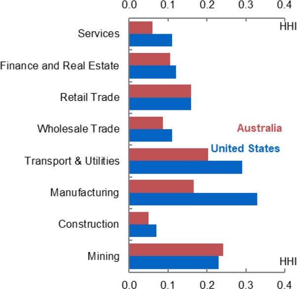
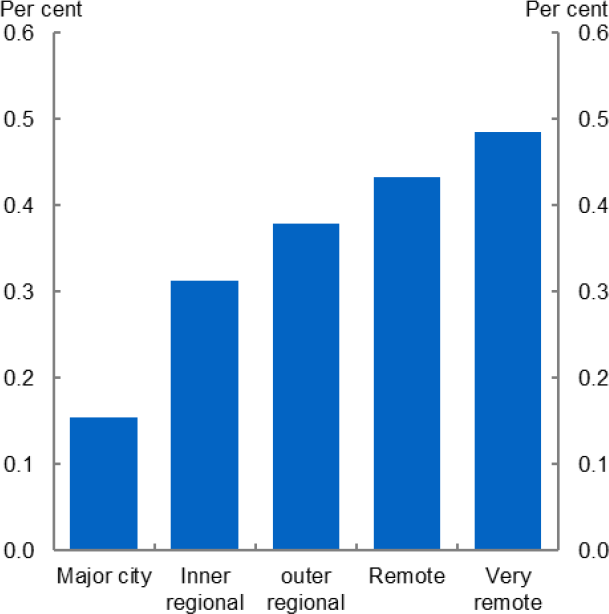
Note: Figure 1, services include Accommodation and Hospitality, Information, Media and Technology, Professional Services, Administrative Services, Arts & Recreation, and Other Services. Interpretation of the results for mining might be affected by fly-in-fly-out work. Figure 2 remoteness based on ABS remoteness structures. Source: Author’s calculations, Rinz (2018)
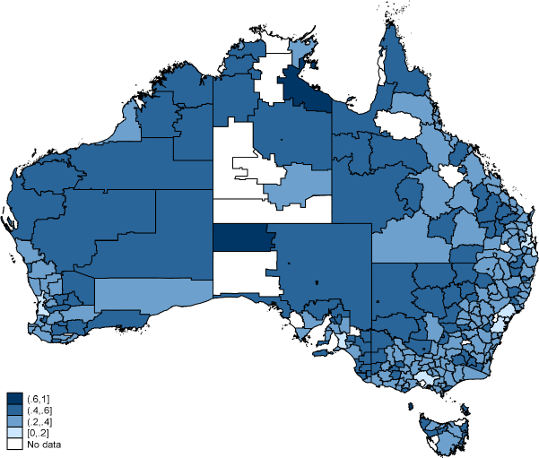
Much of the variation also reflects geographic differences. As shown in Figure 2, markets in major cities tend to be less concentrated. Unsurprisingly, regional and rural areas tend to have more concentrated labour markets.
Overall, local labour market concentration has not changed in Australia over the sample. Figure 3 plots the average level of concentration. Using an employment-weighted average of the individual labour markets shows some decline over the period. However, this reflects a compositional shift with workers moving to urban centres, which tend to be less concentrated. The unweighted average has been broadly unchanged (Figure 3), while the distribution has been similarly stable (Figure 4). Taken together, this shows that concentration has been broadly unchanged over the period.
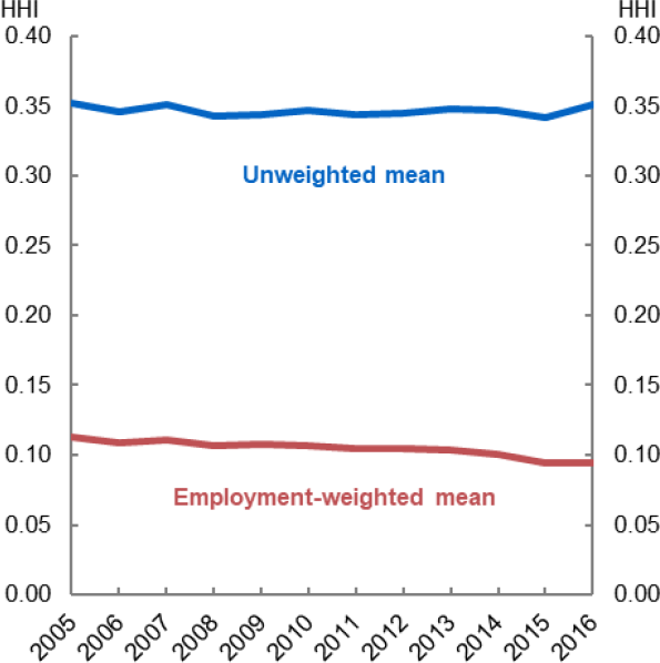
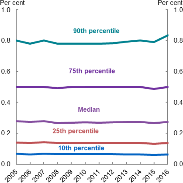
Source: Author's calculations
5. Wages and concentration
While there is no evidence of a general increase in concentration in Australian labour markets, the relationship between concentration and wages is still relevant. Given such a relationship should exist in theory, its presence would indicate that the measure of concentration has some economic signal, and so would be worth tracking.
As noted earlier, other factors could be important in mitigating or amplifying the effect of labour market concentration on wages. As such, we might need to take account of these additional factors in considering whether labour market concentration has weighed on wages in recent years, rather than just examining aggregate concentration levels.
To provide some initial evidence on the relationship between concentration and wages, Figure 5 plots changes in the HHI index over the sample for labour markets against their average annual real wages growth. Real wages growth has tended to be higher in local labour markets where the HHI has declined, providing some initial evidence that local labour market concentration is associated with lower wages.
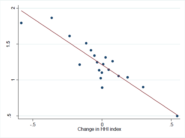
Note: Plots changes in HHI in local labour markets against the average growth in their real wages over the sample. Dots are average for buckets of firms, line is line of best fit.
Source: Author's calculations
5.1. Model specification and identification
To test this more formally, I now turn to a regression framework. In specifying the regression, it is important to think about how wages are set.
As discussed in Manning (2021), in many models of labour market power the firm optimally sets its wages some fraction below its marginal revenue product of labour (MRPL, closely linked to productivity). The extent of this markdown will be a function of the firm's market power (the elasticity of its labour supply curve ). As such, these models predict that the wage (for the market or firm) can be written as:[7]
In our case, the market power is summarised by the measure of concentration. The degree of market power could be market specific, or firm specific, depending on the model.
This set-up leads to our first two models:
- Monopsonistic competition: Wages are set as markdown on the MRPL, with this markdown being the same for all firms and being related to the market concentration. This is the standard regression framework used in most papers (Rinz 2018; Azar et al 2020).
- Oligopsony: As a simple extension, we can allow the degree of market power to vary with plant size . In this case the markdown differs based on the plant's power, which is related to its market share. This oligopsonistic framework is more in line with recent papers such as Berger et al (2021).
In each case, the coefficient of interest is .
For both models Xi,t contains several controls, including industry-by-time and location-by-time effects, and market size. These controls help us to strip out factors affecting all firms or markets, such as local or industry demand, and focus on changes in concentration that reflect changes in market power for the market or firm. Potential examples of such changes include: an exogenous change in the number of competitors (such as due to M&A); technological changes in the ease of finding jobs; and changes in workers' views of the substitutability of different employers, such as differences in cultures.
Some papers use instruments to help identify exogenous changes in market power/supply elasticity. The key concern is that some shocks can affect wages both by impacting the MRPL, as well by changing the concentration and labour supply elasticity and, therefore, markdown. If no measure of productivity is included both effects will be attributed to concentration.
This concern is lessened somewhat because I include a measure of productivity. Still, as productivity measurement is imperfect, I also estimate a version of the monopsony model where I use an instrument for concentration. Specifically, I use the average of the (inverse of the) number of plants in the industry in other locations, with each location being weighted by its share of industry employment. This approach is used in a number of papers (such as Azar et al 2020). The use of the number of firms, rather than the HHI, should lessen the impact of shocks to individual firms, while focusing on national changes allows us to abstract from local shocks. That said, this approach makes it difficult to include industry by time effects, and so is not the preferred specification.[8]
Several recent models have also argued that the degree of market concentration can affect the pass-through of firm-level productivity shocks onto wages. In oligopolistic models such as by Berger et al (2021) and Benmelech et al (2022), increases in productivity, which make the firm larger, move it onto a steeper part of the labour supply curve. As such the markdown increases, leading wages to increase by less than productivity, meaning the pass-through to wages is incomplete. Moreover, the degree of pass-through tends to decline as firms become larger, and as such pass-through becomes a function of firms' market shares. Such a specification also naturally comes out of some search-and-match based models of the labour market (Jarosch et al 2019).
Examining the impact on pass-through is interesting, given evidence of declining productivity pass-through in Andrews et al (2019). As such, I also use a third rent-sharing specification:
- Rent sharing: The pass-through of productivity is a function of the labour market power and, therefore, concentration. This could be plant-level or market-level concentration:
Xi,t contains similar controls. In this case we can also include local market by time fixed effects, given the focus is not on the interaction between concentration and productivity.
5.2. Baseline results
Table 2 shows the results from the monopsony model. Running the model at the local labour market level (Local Labour Market model), we can see that increases in concentration are associated with lower wages, consistent with expectations. The coefficient is larger using the instrumental variable. This suggests that changes in the local HHI driven by national-level variation in concentration have a larger impact on wages and provide additional support to the baseline findings.
| Local Labour Market model | Plant-level model | ||||
|---|---|---|---|---|---|
| Monopsony | Monopsony – IV | Monopsony | Monopsony – IV | Oligopsony | |
| Productivity | 0.077*** (0.001) |
0.070*** (0.002) |
0.153*** (0.004) |
0.153*** (0.001) |
0.158*** (0.004) |
| Concentration – HHI | −0.122*** (0.008) |
−0.542** (0.253) |
−0.005 (0.011) |
−0.021** (0.009) |
|
| Concentration – plant market share | −0.103*** (0.027) |
||||
| R2 | 0.67 | 0.009 | 0.781 | 0.042 | 0.801 |
| N | 302,000 | 302,000 | 3,660,000 | 3,660,000 | 3,560,000 |
| Fixed effects | |||||
| Local market | Y | Y | Y | Y | N |
| Time*Industry | Y | N | Y | N | N |
| Time*Location | Y | Y | Y | Y | N |
| Time*Market | N | N | N | N | Y |
| Plant | N | N | Y | Y | Y |
| Note: All models contain controls for market size (number of workers in the market), and plant-level models account for number of plants in the parent firm. | |||||
The relationship is weaker if we regress plant-level wages on local labour market concentration (Plant-level monopsony models). This may reflect the fact that the model has difficulty accounting for plant-level variation in wages (and markdowns) using the market-level concentration metric. This suggests that the monopsony model might not be ideally suited to explaining firm-level wages.
The final column shows the results from the oligopsonistic model, where the concentration metric is the plant's share of employment in the local labour market. We see a significant negative relationship, consistent with firms setting a larger markdown and, therefore, lower wage, as they gain market share. This is the case even after accounting for market-level concentration, which will be captured in the fixed effect structure. So even within markets there is a great deal of variation in market power and markdowns.
Finally, Table 3 shows the results from the rent-sharing model. In all cases, pass-through from productivity to wages declines when concentration rises. Of particular interest, Column 3 shows the results when accounting both for market- and firm-level concentration. It shows that in more concentrated markets pass-through tends to be lower. But even within these markets there is variation, with larger firms having even lower pass-through.
| HHI | Firm Share | Both | |
|---|---|---|---|
| Productivity | 0.170*** (0.005) |
0.161*** (0.004) |
0.170*** (0.004) |
| Local Concentration (HHI)* Productivity | −0.194*** (0.016) |
−0.174*** (0.017) |
|
| Plant Concentration (plant share)* Productivity | −0.163*** (0.011) |
−0.074*** (0.01) |
|
| R2 | 0.797 | 0.796 | 0.797 |
| N | 3,560,000 | 3,560,000 | 3,560,000 |
| Fixed effects | |||
| Time*Market | Y | Y | Y |
| Plant | Y | Y | Y |
| Note: All regressions include a set of common controls covering firm characteristics (number of plants in the firm) and market characteristics (number of workers in the market). Errors clustered at the local market level. | |||
Figure 6 provides a sense of the magnitude of these results. Focusing first on the regressions using market concentration, wages are on average 4½ per cent lower in a highly concentrated industry (75th percentile HHI of 0.5), compared to a low concentration industry (25th percentile HHI 0.15). Equally, the degree of rent-sharing (the share of productivity changes passed on to wages) is around 1¾ percentage points lower in a high concentration industry. But gaps don't just exist across markets. Even within markets there is a great deal of difference between high and low market share firms. High market share firms pay wages that are 2 per cent lower (once accounting for differences in productivity and other factors), and the share of productivity passed on to wages for large firms is around 1½ percentage points lower.
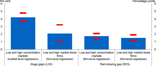
Note: Low and high concentration markets are the 25th and 75th percentile, respectively, and these differ across market versus firm specification due to differing firm counts per market. Low market share is zero, high market share is 20 per cent of market (95th percentile). Results from headcount models, either market-level or firm-level, as indicated. Red dashes show two standard deviation range of estimates.
Source: Author's calculations
This latter finding highlights the importance of firm heterogeneity when considering local labour market power. It also suggests that aggregate concentration measures may not be sufficient to consider changes in local labour market power. Instead, we may need to consider the full distribution of market shares, and how they have changed, to properly understand changes in market power and implications for wages.
5.3. Subsample results
As noted above, the degree of labour market concentration has been unchanged over the sample. At first blush, this would suggest that concentration cannot explain low wages growth pre-COVID. However, papers such as Benmelech et al (2022) have found evidence that the impact of given levels of concentration can change over time.
To examine this, I run the baseline market-level regression, but allowing all coefficients to vary across three financial year sub-samples: 2005–2007; 2008–2010 (GFC); 2011–2015 (post-GFC). This will allow me to consider whether the impacts of HHI on wages have increased, even if concentration has remained unchanged.[9]
Table 4 shows the results of the sub-sample regression. The impact of concentration more than doubled from the early period to the 2011–2015 period.[10]
| Baseline | Sub-sample | National Unemployment | State Unemployment | |
|---|---|---|---|---|
| Concentration | −0.122*** (0.008) |
−0.067*** (0.020) |
−0.123*** (0.015) |
−0.122*** (0.015) |
| Concentration * GFC | −0.076*** (0.021) |
|||
| Concentration * Post GFC | −0.079*** (0.022) |
|||
| Concentration * Unemployment | −0.359 (1.557) |
−0.035 (1.106) |
||
| R2 | 0.67 | 0.67 | 0.67 | 0.67 |
| N | 302,000 | 302,000 | 302,000 | 302,000 |
| Fixed effects | ||||
| Local market | Y | Y | Y | Y |
| Time*Industry | Y | Y | Y | Y |
| Time*Location | Y | Y | Y | Y |
| Note: All regressions include a set of common controls covering market characteristics (number of workers in the market). For GFC models, all controls other than firm FE are interacted with period dummies. Pre-GFC is 2005–2007. GFC is 2008–2010. Post GFC is 2011 to 2015. For unemployment models, interacting unemployment with productivity does not change the results. Errors clustered at the local market level. | ||||
One potential explanation could be softer labour markets. In many search-and-match models a tighter labour market leads to greater bargaining power for workers given the greater chance of finding another job, which could lower the impact of concentration. However, this does not appear to be the case, as there is no significant evidence that the impacts of concentration on wages are stronger when the labour market is weaker, as measured by the national or state-level unemployment rate (Columns 3 and 4).
To put the sub-sample result in perspective, Figure 7 shows the estimated wage gap between a high and low concentration markets for the early and recent periods. This gap is around to 2 per cent in the early period, but 5 per cent in the more recent period.
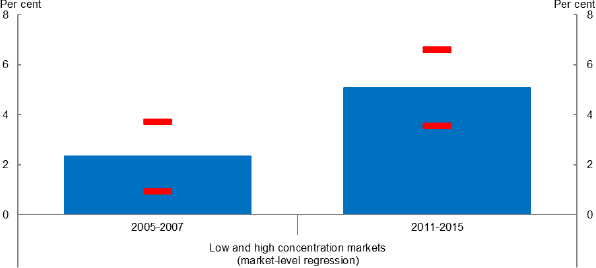
Note: Low and high concentration markets are the 25th and 75th percentile, respectively. Results from headcount models estimated at the market level shown over sub-samples in Table 5. Dashes show two standard deviation confidence interval. Interval for post period simply based on standard error of interaction term.
Source: Author's calculations
To get a sense of the macroeconomic impacts I use a simple back of the envelope calculation. The national employment-weighted average HHI is around 0.1. Multiplying this by the change in the HHI coefficient between periods (0.80) suggests that nationally wages were around 0.80 per cent lower than they would have been on average from 2011–2015, compared to the case whether the coefficient did not change. Given estimates put the ‘unexplained’ weakness in wages growth at around 0.25 per cent per year (Cassidy 2019), this suggests that the increasing impact of concentration can account for a large portion of the weakness in wages growth pre-COVID.
Obviously, the calculation is very simple and does not account for heterogeneity in outcomes or general equilibrium mechanisms. As such it should not be interpreted precisely. But it does suggest that the increasing impact of concentration has had a substantial effect on aggregate wages.
6. Why has the impact of concentration increased?
A key question from a policy standpoint is, why has the impact of concentration increased? Understanding this is crucial in identifying what, if any, polices could and should be implemented to offset the apparent increase in market power.
I examine three potential explanations motivated by the existing literature on firm dynamism and labour market concentration:
- Declining industry or occupational mobility
- Declining firm dynamism and entry
- Declining union membership.
6.1. Declining occupational mobility
One explanation I examine is declining occupational or industry mobility. Much of the work on labour market concentration assumes that workers cannot move between local labour markets due to geographic or skill barriers. However, in practice workers can move between geographies, industries or occupations, even if it is costly or difficult. If it becomes easier to move between these markets, and so the set of potential outside options becomes larger, the effect of concentration within the market might become smaller.
For example, in the Berger et al (2021) model they allow for differentiation in supply of labour across, as well as within industries. When differentiation across industries declines, consistent with easier mobility across industries, the impact of differentiation and concentration within industries is lessened.
Schubert et al (2021) focus on this issue empirically. They derive a model where workers can potentially move to other industries in their locality. They show that in this case wages will be impacted by the ‘outside options’ that other occupations in their locality represent. Failing to include these outside options can bias the estimated impact of the HHI on wages. Similarly, they show that the impact of labour market concentration on wages tends to be smaller in industries with more cross-industry mobility, and the outside options become more important.
Declining occupational mobility and increasing frictions in moving between industries and occupations may be relevant in the Australian case. For example, Figure 8 shows that a moderate portion of the decline in job-to-job switching (as defined in Deutscher 2019) reflects fewer people changing occupations. This might suggest increasing frictions between labour markets.
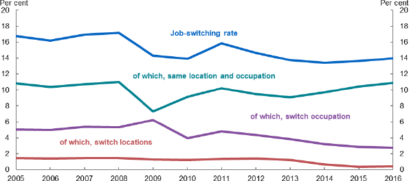
Note: Job-to-job switching as defined in Deutscher (2019). Location defined as SA4 or greater capital city area. Occupation is 2-digit ANZSCO.
Source: Author's calculation
To consider this, I include the measure of outside options suggested by Schubert et al (2021) and examine the impact on the coefficient on the HHI in the full sample, and in the sub-sample regressions.
The outside-option variable is constructed as a weighted average of the wages for firms in all other industries in the local area. The weights are a function of two factors: the share of employment for each of these industries in the local area (excluding the base industry), to capture how ‘important’ each industry is in the local area; and the national rate of switching between the base and the other industry (measured as a share of job-switchers only), to capture the ease with which people can move from the base industry to the alternative industry.[11]
The results of the regression are contained in Table 5. Focusing on Column 2, we can see that having strong outside options leads to higher wages. Moreover, the effect of concentration within a market is lower in this regression, suggesting that failing to account for these options can cause us to overstate the effects of the HHI.
Focusing on the sub-sample in Column 3, we see outside options becoming less impactful over time. This is consistent with what we might expect to see if it became harder to move between industries. This suggests that declining occupational mobility may have weighed on wages growth by limiting workers' ability to leverage options outside their industries in wage negotiations, which would be consistent the findings in Deutscher (2019) that areas with less job switching tend to see lower wages growth.
| Baseline | With OO | Sub-sample OO | |
|---|---|---|---|
| Concentration | −0.122*** (0.008) |
−0.104*** (0.014) |
−0.047** (0.020) |
| Outside option | 0.040*** (0.004) |
0.050*** (0.004) |
|
| Concentration * GFC | −0.076*** (0.021) |
||
| Concentration * Post GFC | −0.083*** (0.021) |
||
| Outside option * GFC | −0.010*** (0.004) |
||
| Outside option * Post GFC | −0.020*** (0.004) |
||
| R2 | 0.670 | 0.671 | 0.671 |
| N | 302,000 | 302,000 | 302,000 |
| Fixed effects | |||
| Local market | Y | Y | Y |
| Time*Industry | Y | Y | Y |
| Time*Location | Y | Y | Y |
| Note: All regressions include a set of common controls covering market characteristics (number of workers in the market). All controls other than firm FE are interacted with period dummies. Pre-GFC is 2005–2007. GFC is 2008–2010. Post GFC is 2011 to 2015. Errors clustered at the local market level. | |||
Still, this regression provides no evidence that changes in the importance of outside options and occupational mobility have increased the impact of concentration. The coefficient on the HHI declines by a similar amount over the sample as in the model without outside options, so changes in the importance of the omitted outside options variable was not driving the decline.
To test more directly the impact of declining occupational mobility on the role of concentration, I extend the baseline market-level monopsony model to incorporate industry switching rates. Specifically:
Switchind,it is the national rate of industry switching in the relevant ANZSIC 3-digit industry. This is either expressed as a share of all job switchers (leave share), or as a share of all job switchers and stayers (leave rate) with both defined as in Deutscher (2019) and focusing on worker's main jobs.
I focus on the national, rather than local rate of switching, to avoid endogeneity between local conditions and switching rates. It also helps to limit noise introduced by very small markets, where rates can be very volatile. Switch rates are demeaned for each industry. As such we are focusing on changes in switching rates and abstracting from structural differences across industries that might affect switching, concentration and wages.
The coefficients of interest in this case are and . If concentration amongst incumbents is less impactful in industries with more occupational switching, the coefficient would be positive. Similarly, if outside options are more important where switching is more prevalent would be positive.
| OO model | OO model with leave share | OO model with leave rate | |
|---|---|---|---|
| Concentration | −0.104*** (0.014) |
−0.104*** (0.014) |
−0.104*** −0.011 |
| Outside option | 0.040*** (0.004) |
0.039*** (0.004) |
0.040*** (0.004) |
| Concentration * Leave share | −0.288* (0.151) |
||
| Outside option * Leave share | 0.086*** (0.032) |
||
| Concentration * Leave rate | 0.035 (0.324) |
||
| Outside option * Leave rate | 0.228*** (0.066) |
||
| R2 | 0.671 | 0.671 | 0.671 |
| N | 302,000 | 299,000 | 302,000 |
| Fixed effects | |||
| Local market | Y | Y | Y |
| Time*Industry | Y | Y | Y |
| Time*Location | Y | Y | Y |
| Note: All regressions include a set of common controls covering market characteristics (number of workers in the market). Leave share captures share of job leavers that change industry. Leave rate captures share of total workers in the industry (leavers and stayers) that change industry. Errors clustered at the local market level. | |||
Using both the leave share and rate, we see no evidence that concentration is less impactful where there is more occupational switching (Table 6). However, there is some evidence that outside options are more important in industries with higher switching rates.
Taken together, these results provide some evidence that decreasing occupation and industry mobility may have weighed on wages pre-COVID by limiting the role of outside options. However, the direct evidence with respect to its role in increasing the impact of concentration is limited.
6.2. Declining firm dynamism
The role of firm entry and dynamism in labour market dynamism has been considered in some recent papers (Bilal et al 2019). In these papers, firms enter and attract staff away from incumbent firms, meaning that declines in firm entry can be associated with lower job-to-job switching and few outside options for workers.
Such dynamics are evident in Australia. Much of the decline in job-to-job switching, as defined in Deutscher (2019), has reflected less workers switching from established mature firms to young firms. And this has coincided with declines in firm entry rates (Figure 9).
These patterns are also evident within local areas. Figure 10 shows that there is a strong positive correlation between firm entry rates in a local area and the rate of job-to-job switching. This is the case even controlling for time-invariant differences across geographies and the overall business cycle. Moreover, this relationship is only evident when focusing on switching between mature and young firms. There is no relationship between firm entry and mobility of workers between mature incumbent firms, indicating that the relationship is not simply driven by local economic conditions (Appendix A).
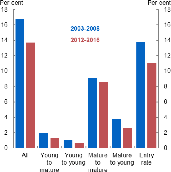
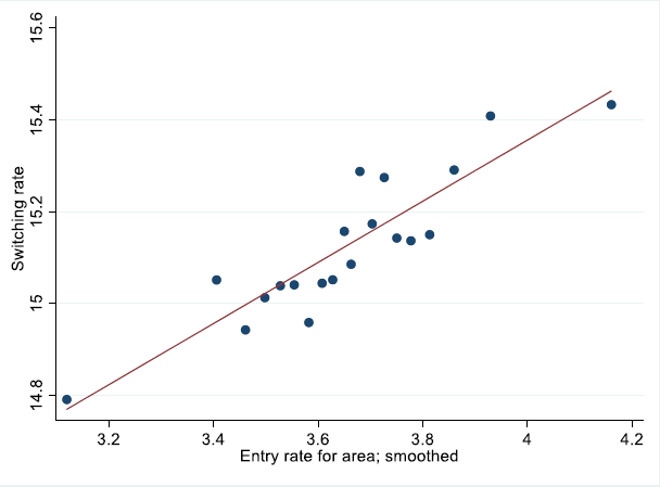
Figure 9 young firms are 0–5, mature firms are older than 5 years. Figure 10 plots entry rates for SA4s or greater capital city areas versus the job-to-job switching rate. This is shown having residualised with respect to time effects, area effects, and the employment share of young firms. Approximately 780 SA4*year combinations based on 120 million workers.
Source: Author's calculations
Taken together, these results suggest that firm entry represents an additional source of competition for labour for incumbents. Entrants could broaden the set of outside option for workers, and so raise their bargaining power. As such, declining firm entry and dynamism could make concentration among incumbents more impactful.
To examine the role of declining firm entry, I extend the baseline market-level monopsony model to incorporate firm entry rates. Specifically:
Entryind,t is the national rate of entry in the relevant ANZSIC 3-digit industry. I again focus on the national, rather than local rate of entry and use demeaned entry rates.
The coefficient of interest in this case is . If concentration among incumbents is less impactful in industries with rising entry, the coefficient would be positive.
Table 7 shows the results of the regression with entry rates constructed using the entries of firms, and entries of plants (recording a firm opening a plant in a new locality as an entry). The results consistently show that, where industry entry rates are higher, local labour market concentration is less impactful.[12] That is, having a high level of firm entry seems to provide an additional source of competition, lessening the market power associated with concentration among incumbents.
| Baseline | Plant-based entry rate | Firm-based entry rate | |
|---|---|---|---|
| Concentration (HHI) | −0.122*** (0.008) |
−0.110*** (0.016) |
−0.111*** (0.015) |
| Concentration (HHI) * Entry Rate | 0.540*** (0.204) |
0.800*** (0.228) |
|
| R2 | 0.67 | 0.683 | 0.686 |
| N | 302,000 | 274,000 | 274,000 |
| Fixed effects | |||
| Local market | Y | Y | Y |
| Time*Industry | Y | Y | Y |
| Time*Location | Y | Y | Y |
| Note: All regressions include a set of common controls covering market characteristics (number of workers in the market. Errors clustered at the local market level. | |||
To provide a sense of the macro importance of declining entry rates I do a similar calculation as for the sub-sample regressions. On average there was around a 5 percentage point decline in the entry rate of plants and firms across the sample. Applying this to the coefficients from Columns 2 and 3 of Table 6 and using the employment-weighted average HHI (0.1), this suggests that wages would have been around 0.250.50 per cent higher in 2015, had entry rates not declined.
Again, the estimate should not be interpreted too precisely as it is a simple, partial equilibrium estimate. But these results do suggest that declining firm entry and dynamism had a substantial negative impact on workers' wages by lowering their bargaining power and increasing the power of incumbent firms.
6.3. Declining union membership
Benmelech et al (2022) argue that declining union membership rates could account for the increased impact of concentration on wages in the US. They argue that unions provide an offset to monopsony power. With lower union membership there is less of an offset, and so concentration could be more impactful.
Union membership rates in Australia have been declining for decades. And while Bishop and Chan (2019) found no evidence that declining union membership led to lower wage outcomes in Enterprise Bargaining agreements in Australia – as the share of agreements with union involvement remained unchanged – it is still worth examining the interaction between union coverage, labour market concentration and wages.
To do so, I run a similar specification to the above, and to that used in Benmelech et al (2022):
Union sharediv,t is the share of employees in each ANZSIC division that are part of a union. This is taken from the ABS Employee Earning, Benefit and Trade Union Membership release for 2006–2013. Unfortunately, more granular industry-level data were not available. Again, rates were demeaned to focus on changes in union membership, rather than the levels.
Table 8 shows the results. There is a significant positive coefficient on , indicating that the impact of market concentration on wages is smaller (in absolute terms) when union membership rates are higher. This does suggest that declining unionisation rates may explain part of the increased impact of concentration on wages. However, declining entry rates appear to be the more important factor, particularly once we try to account for both entry and union coverage (Column 3).
More generally, it is important to keep in mind that these models only capture one mechanism through which union coverage can affect wages. They do not account for any other effects changes in union membership rates could have on the economy, in terms of productivity, employment or output, and do not speak more broadly to the net benefits or costs of lower union membership. They simply indicate that, in the presence of monopsony power stemming from concentrated labour markets, collective worker bargaining can play an offset, and that this offset may have declined over time.
| Baseline | Union | Union and Entry | |
|---|---|---|---|
| Concentration | −0.133*** (0.016) |
−0.144*** (0.016) |
−0.127*** (0.018) |
| Concentration * Entry Rate | 0.939*** (0.254) |
||
| Concentration * Union | 0.009** (0.004) |
0.005 (0.004) |
|
| R2 | 0.67 | 0.70 | 0.70 |
| N | 247,000 | 219,000 | 219,000 |
| Fixed effects | |||
| Local market | Y | Y | Y |
| Time*Industry | Y | Y | Y |
| Time*Location | Y | Y | Y |
| Note: All regressions include a set of common controls covering market characteristics (number of workers in the market and market fixed effects). Regressions 2006–2013. Errors clustered at the local market level. | |||
One related explanation not explored in detail due to data constraints is changes in the share of workers on different pay-setting mechanisms. To the extent that pay is set nationally for a firm or industry, local concentration may be less impactful. This does not necessarily mean that wages will be higher, but the relationship between local concentration and wages may be weaker.
Unfortunately, data on pay-setting shares by ANZSIC division are only available for three years across my sample: 2008, 2012 and 2014. Based on this limited data, there is cross-sectional evidence that the HHI is more impactful in divisions with higher use of individual agreements. However, it is possible that this is driven by some common factor affecting both, such as level of education required for staff. Focusing within sectors, there is no evidence that the HHI has become relatively more impactful where the individual agreements usage increased.[13]
With additional data this channel could be assessed more directly. However, given wages in individual agreements have to be at least as high as award wages, and given that individual agreement usage increased up to 2008, but then fell, increased use of individual awards seems unlikely to be behind the results in this paper.
7. Conclusion
Wages growth was surprisingly low during the pre-COVID period. Understanding whether or what structural factors caused this weakness is crucial, given they may continue to weigh on wages in the post-COVID period. This would have implications for inflation, government revenues and worker welfare.
Overall, this paper has demonstrated that the increasing impact of labour market concentration may have weighed on wages growth pre-COVID, subtracting a bit under 1 per cent from wages on average from 2011–2015. This is the case even though concentration itself did not increase.
A key driver of the increased impact of concentration appears to be declining firm entry and dynamism, as it has meant that incumbents faced less competition from new entrants, allowing them to exert more market power for given concentration levels. Declining occupational mobility and union coverage may have also played some role, but declining entry appear to be the major driver.
These results highlight a second, direct channel through which declining firm entry, dynamism and competitive pressure have weighed on wages growth. They sit alongside earlier work showing an indirect channel through which declining dynamism weighed on wages: by lowering productivity growth (Andrews and Hansell 2021; Andrews et al 2022; Hambur forthcoming). As such, these results further motivate an ongoing focus on potential obstacles to firm entry, growth and dynamism, as well as labour market frictions, in developing policies to drive better outcomes for workers and economic growth.
References
Abel W, S Tenreyro and G Thwaites (2018), ‘Monopsony in the UK’, Centre for Economic Policy Research Discussion Paper DP13265.
Andrews D, N Deutscher, J Hambur and D Hansell (2019), ‘Wage Growth in Australia: Lessons from Longitudinal Microdata’, Australian Treasury Working Paper No 2019-04.
Andrews D, J Hambur, D Hansell and A Wheeler (2022), ‘Reaching for the Stars: Australian Firms and the Global Productivity Frontier’, Australian Treasury Working Paper No 2022-01.
Andrews D and D Hansell (2021), ‘Productivity-enhancing Labour Reallocation in Australia’, Economic Record, 97(317), pp 157–169.
Arsov I and R Evans (2018), ‘Wage Growth in Advanced Economies’, Reserve Bank of Australia Bulletin, March.
Australian Treasury (2017), ‘Analysis of Wage Growth’, Technical Paper, November.
Azar J, I Marinescu, M Steinbaum and B Taska (2020), ‘Concentration in US Labor Markets: Evidence from Online Vacancy Data’, Labour Economics, 66, Article 101886.
Benmelech E, NK Bergman and H Kim (2022), ‘Strong Employers and Weak Employees: How Does Employer Concentration Affect Wages?’, The Journal of Human Resources, 57(S), pp S200–S250.
Berger D, K Herkenhoff and S Mongey (2021), ‘Labor Market Power’, Becker Friedman Institute for Economics Working Paper No 2021–58.
Bilal AG, N Engbom, S Mongey and GL Violante (2019), ‘Firm and Worker Dynamics in a Frictional Labor Market’, NBER Working Paper No 26547.
Bishop J and I Chan (2019), ‘Is Declining Union Membership Contributing to Low Wages Growth?’, Reserve Bank of Australia Research Discussion Paper No 2019–02.
BITRE (Bureau of Infrastructure, Transport and Regional Economics) (2018), ‘Working Zones 2016’, BITRE Information Sheet 98.
Cassidy N (2019), ‘Low Wage Growth in Australia – An Overview’, Paper presented at the annual RBA conference on ‘Low Wage Growth’, Sydney, 4–5 April.
De Loecker J, J Eeckhout and G Unger (2020), ‘The Rise of Market Power and the Macroeconomic Implications’, The Quarterly Journal of Economics, 135(2), pp 561–644.
Deutscher N (2019), ‘Job-to-Job Transitions and the Wages of Australian Workers’, Treasury Working Paper No 2019–07.
Hambur J (forthcoming), ‘Product Market Competition and Its Implications for the Australian Economy’, Economic Record.
Handwerker EW and M Dey (2022), ‘Some Facts about Concentrated Labor Markets in the United States’, U.S. Bureau of Labor Statistics BLS Working Paper No 550.
Jarosch G, JS Nimczik and I Sorkin (2019), ‘Granular Search, Market Structure, and Wages’, NBER Working Paper No 26239, rev May 2020.
Lipsius B (2018), ‘Labor Market Concentration Does Not Explain the Falling Labor Share’, Job Market Paper, University of Michigan, November. Available at <https://ideas.repec.org/p/jmp/jm2018/pli1202.html>.
Lowe P (2018), ‘Productivity, Wages and Prosperity’, Address to the Australian Industry Group, Melbourne, 13 June. Available at <https://www.rba.gov.au/speeches/2018/sp-gov-2018-06-13.html>.
Manning A (2021), ‘Monopsony in Labor Markets: A Review’, ILR Review, 74(1), pp 3–26.
Marinescu I, I Ouss and L-D Pape (2021), ‘Wages, Hires, and Labor Market Concentration’, Journal of Economic Behavior & Organization, 184, pp 506–605.
Moscarini G and F Postel-Vinay (2017), ‘The Relative Power of Employment-to-Employment Reallocation and Unemployment Exits in Predicting Wage Growth’, The American Economic Review, 107(5), pp 364–368.
OECD (Organisation for Economic Co-operation and Development) (2020), Competition in Labour Markets, Background Note, OECD, Paris. Available at <https://www.oecd.org/daf/competition/competition-concerns-in-labour-markets.htm>.
OECD (2021), The Role of Firms in Wage Inequality: Policy Lessons from a Large Scale Cross-Country Study, OECD Publishing Press, Paris.
Rinz K (2018), ‘Labor Market Concentration, Earnings Inequality, and Earnings Mobility’, U.S. Census Bureau Center for Administrative Records Research and Applications, CARRA Working Paper 2018–10.
Schubert G, A Stansbury and B Taska (2021), ‘Employer Concentration and Outside Options’, Washington Center for Equitable Growth Working Paper, rev March 2022.
U.S. Department of Justice and Federal Trade Commission (2010), ‘Horizontal Merger Guidelines’. Available at <https://www.justice.gov/atr/merger-enforcement>.
Appendix A: Additional charts and tables
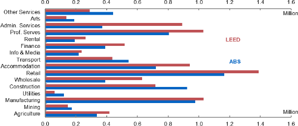
Notes: ABS data is from Labour Force Survey detailed and is on a person basis. LEED is on a job basis. As such, sectors with high rates of multiple-job holdings like retail are larger in LEED. LEED also excludes self-employed, which may be more important in construction. The higher employment in Administrative Services reflects differences in how employment in labour hire and employment services are captured in tax data (often via the service providers), compared to in labour statistics (often via the end employer).
Source: Author's calculations; ABS
| Unweighted | Weighted | |
|---|---|---|
| 25th percentile | 0.186 | 0.011 |
| Median | 0.363 | 0.031 |
| Mean | 0.401 | 0.103 |
| 75th percentile | 0.584 | 0.133 |
| Note: Reports summary statistics for local labour markets. Average taken for each market across 2005–2016. | ||
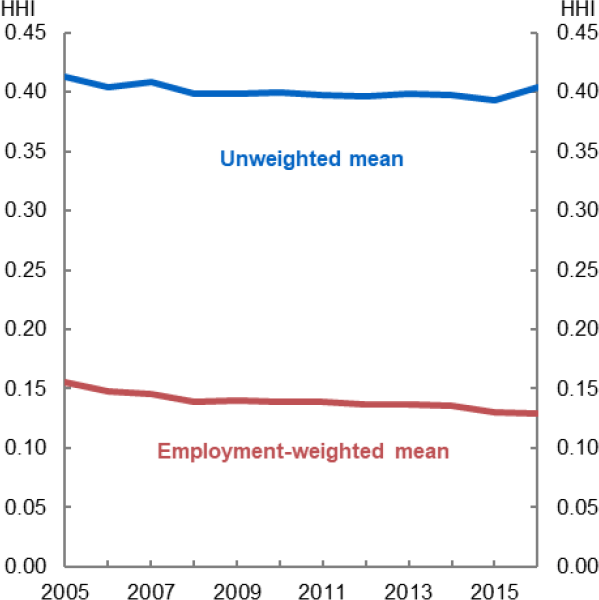
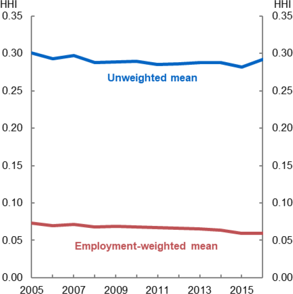
Source: Author's calculations
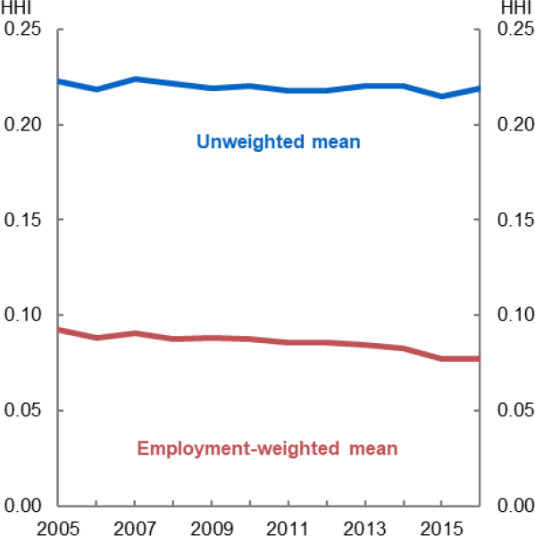
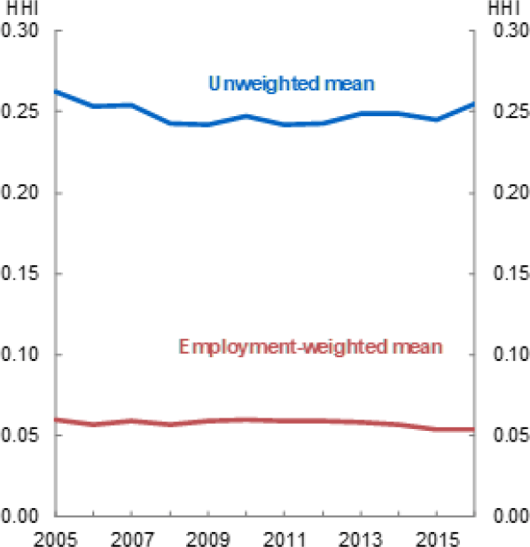
Source: Author's calculations
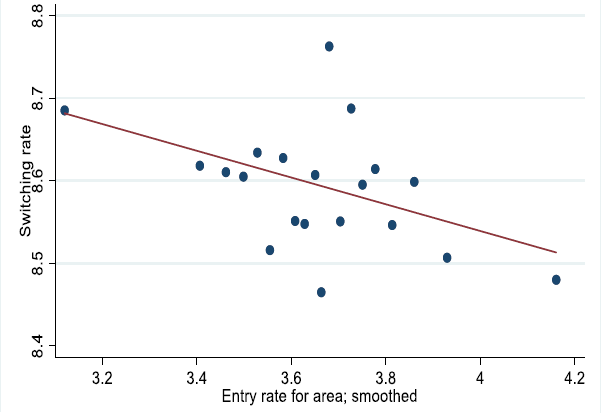
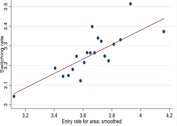
Note: Plots entry rates for SA4s or greater capital city areas versus the job-to-job switching rate. This is shown having residualised with respect to time effects, area effects, and the employment share of young firms. Approximately 780 SA4*year combinations based on 120 million workers.
Source: Author's calculations
Appendix B: Regression robustness results
| Headcount | Wages | |||||
|---|---|---|---|---|---|---|
| None | Local | Time trends | None | Local | Time trends | |
| Concentration (HHI) | −0.162*** (0.012) |
−0.153*** −0.015 |
−0.122*** (0.014) |
−0.238*** (0.012) |
−0.359*** (0.015) |
−0.311*** −0.025 |
| Productivity | 0.175*** (0.002) |
0.087*** (0.002) |
0.077*** (0.002) |
0.174*** (0.004) |
0.085*** (0.002) |
0.075*** (0.002) |
| R2 | 0.107 | 0.631 | 0.671 | 0.110 | 0.633 | 0.672 |
| N | 306,000 | 302,000 | 302,000 | 306,000 | 302,000 | 302,000 |
| Fixed effects | ||||||
| Local market | N | Y | Y | N | Y | Y |
| Time*Industry | N | N | Y | N | N | Y |
| Time*Location | N | N | Y | N | N | Y |
| Note: All regressions include a set of common controls covering market characteristics (number of workers in the market). Errors clusters at the local market level. | ||||||
| Headcount | ||||||
|---|---|---|---|---|---|---|
| None | Local | Ind area time | Plant | Local time | All | |
| Productivity | 0.371*** (0.005) |
0.318*** (0.05) |
0.316*** (0.05) |
0.164*** (0.004) |
0.324*** (0.05) |
0.170*** (0.05) |
| Local Concentration (HHI)* Productivity | −0.207*** (0.016) |
−0.233*** (0.014) |
−0.239*** (0.015) |
−0.122*** (0.011) |
−0.286*** (0.017) |
−0.174*** (0.017) |
| Firm Concentration (HHI)* Productivity | −0.121*** (0.010) |
−0.201*** (0.008) |
−0.203*** (0.008) |
−0.008 (0.007) |
−0.322*** (0.010) |
−0.322*** (0.010) |
| R2 | 0.211 | 0.326 | 0.344 | 0.781 | 0.367 | 0.797 |
| N | 3,970,000 | 3,970,000 | 3,970,000 | 3,660,000 | 3,860,000 | 3,560,000 |
| Fixed effects | ||||||
| Local market | N | Y | Y | Y | Y | Y |
| Time*Industry | N | N | Y | Y | N | Y |
| Time*Location | N | N | Y | Y | N | Y |
| Time*Market | N | N | N | N | Y | Y |
| Plant | N | N | N | Y | N | Y |
| Note: All regressions include a set of common controls covering market characteristics (number of workers in the market). Errors clusters at the local market level. | ||||||
| Headcount | ||||||
|---|---|---|---|---|---|---|
| Baseline | No small markets (<10 plants) |
Lagged HHI | No rural | No primary industries | ||
| Concentration (HHI) | −0.122*** (0.014) |
−0.135*** −0.028 |
−0.087*** (0.013) |
−0.131*** (0.015) |
−0.144*** (0.016) |
|
| Productivity | 0.077*** (0.002) |
0.031*** (0.002) |
0.077*** (0.002) |
0.076*** (0.002) |
0.073*** (0.002) |
|
| R2 | 0.670 | 0.856 | 0.67 | 0.670 | 0.655 | |
| N | 302,000 | 117,000 | 302,000 | 277,000 | 261,000 | |
| Fixed effects | ||||||
| Local market | Y | Y | Y | Y | Y | |
| Time*Industry | Y | Y | Y | Y | Y | |
| Time*Location | Y | Y | Y | Y | Y | |
| Note: All regressions include a set of common controls covering market characteristics (number of workers in the market). Errors clusters at the local market level. | ||||||
| Headcount | ||||||
|---|---|---|---|---|---|---|
| Baseline | Top 4 share | Top 10 share | Log HHI | |||
| Concentration (HHI) | −0.122*** (0.014) |
−0.122*** (0.018) |
0.014 (0.026) |
−0.146*** (0.005) |
||
| Productivity | 0.077*** (0.002) |
0.078*** (0.002) |
0.077*** (0.002) |
0.077*** (0.002) |
||
| R2 | 0.670 | 0.670 | 0.670 | 0.670 | ||
| N | 302,000 | 302,000 | 302,000 | 277,000 | ||
| Fixed effects | ||||||
| Local market | Y | Y | Y | Y | ||
| Time*Industry | Y | Y | Y | Y | ||
| Time*Location | Y | Y | Y | Y | ||
| Note: All regressions include a set of common controls covering market characteristics (number of workers in the market. Errors clusters at the local market level. | ||||||
| Headcount | ||||
|---|---|---|---|---|
| Industry/occupation | ANZSIC 3-digit | ANZSIC 2-digit | ANZSIC 3-digit | ANZSIC 2-digt and ANZSCO 2 digit |
| Location | Working Zone | Working Zone | SA4/Greater capital area | Working Zone |
| Concentration (HHI) | −0.122*** (0.014) |
−0.115*** (0.020) |
−0.073*** (0.033) |
−0.810*** (0.025) |
| Productivity | 0.077*** (0.002) |
0.064*** (0.002) |
0.049*** (0.003) |
0.062*** (0.002) |
| R2 | 0.670 | 0.677 | 0.779 | 0.672 |
| N | 302,000 | 165,000 | 91,000 | 1,740,000 |
| Fixed effects | ||||
| Local market | Y | Y | Y | Y |
| Time*Industry | Y | Y | Y | Y |
| Time*Location | Y | Y | Y | Y |
| Note: All regressions include a set of common controls covering market characteristics (number of workers in the market. Errors clusters at the local market level. | ||||
| Local Labour Market models | Plant-level model | |||||
|---|---|---|---|---|---|---|
| Labour market | Labour market -Over time | Plant monopsony | Plant oligopsony | Plant rent-sharing | ||
| Market Concentration (HHI) | −0.311*** (0.008) |
−0.246*** (0.023) |
−0.279*** (0.011) |
|||
| Market Concentration GFC (HHI) | −0.085*** (0.021) |
|||||
| Market Concentration post GFC (HHI) | −0.094*** (0.021) |
|||||
| Local Concentration – (plant share) | 3.300*** (0.032) |
|||||
| Local Concentration (plant share)* Productivity | −0.117*** (0.015) |
|||||
| Firm Concentration (plant share)* Productivity | −0.259*** (0.01) |
|||||
| R2 | 0.672 | 0.67 | 0.781 | 0.801 | 0.802 | |
| N | 302,000 | 302,000 | 3,660,000 | 3,560,000 | 3,560,000 | |
| Fixed effects | ||||||
| Local market | Y | Y | Y | N | N | |
| Time*Industry | Y | N | Y | N | N | |
| Time*Location | Y | Y | Y | N | N | |
| Time*market | N | N | N | Y | Y | |
| Plant | N | N | Y | Y | Y | |
| Note: All regressions include a set of common controls covering market characteristics (number of workers in the market) Plant-level model contain control for number of plants in parent firm. Errors clusters at the local market level. | ||||||
| Entry models | Union models (2005-2013) | ||||
|---|---|---|---|---|---|
| Baseline | Plant-based entry rate | Firm-based entry rate | Baseline | Union | |
| Concentration | −0.122*** −0.008 |
−0.110*** −0.016 |
−0.111*** −0.015 |
−0.315*** (0.016) |
−0.322*** (0.016) |
| Concentration * Entry Rate | 0.540*** −0.204 |
0.800*** −0.228 |
|||
| Concentration * Union | 0.010** (0.003) |
||||
| R2 | 0.67 | 0.683 | 0.686 | 0.985 | 0.701 |
| N | 302,000 | 274,000 | 274,000 | 247,000 | 217,000 |
| Fixed effects | |||||
| Local market | Y | Y | Y | Y | Y |
| Time*Industry | Y | Y | Y | Y | Y |
| Time*Location | Y | Y | Y | Y | Y |
| Note: All regressions include a set of common controls covering market characteristics (number of workers in the market) Plant-level model contain control for number of plants in parent firm. Errors clusters at the local market level. | |||||
Acknowledgements
This work was completed through contributions of resources from Treasury's Macroeconomic Group and the Reserve Bank of Australia's Economic Research Department. I would like to thank Cyrille Schwellnus, Dan Andrews, Jeff Borland, Sephorah Mangin, and seminar participants at the RBA, the RBA Quantitative Macroeconomics workshop, the OECD, Treasury and the ATO ALIFE Conference for their helpful comments. The views expressed in this paper are those of the authors and do not necessarily reflect those of The Australian Treasury, the Reserve Bank of Australia or the Australian Government.
This paper is being jointly released by The Australian Treasury as Treasury Working Paper 2023-01. Reflecting this joint release, the paper has remained formatted as in the Treasury version.
Footnotes
More precisely, it reflects the elasticity of the labour supply curve facing the firm. If the curve is not perfectly elastic, the firm can offer a lower wage whilst still attracting some workers. [1]
For a more detailed literature review, see Manning (2021). [2]
Berger et al (2021) derive a general equilibrium model with finite firms and inelastic labour supply across and within firms, which leads to similar conclusions. [3]
An extension would be to use data-driven industry groupings based on flows as in Jarosch et al (2019). [4]
Where firms have complex tax reporting structures, I collapse them down to a single reporting unit. [5]
Some caution should be taken in interpreting the mining results, given the use of fly-in, fly-out (FIFO) workers. Results for construction may also be affected by the prevalence of contractors who will not be recorded as employees. [6]
Search and match models such as Schubert et al (2021) also often reduce to such a characterisation. [7]
Results are also robust to using the lagged HHI to abstract from contemporaneous shocks. See Appendix B. Another approach would be to try to instrument using some ‘direct’ measure of changes in competition, such as mergers. However, such data are not available. [8]
These results are robust to changing the period definition. Note market fixed effects are not allowed to differ across samples, so variation in wages and HHI across sample periods is allowed to affect the results. So, we are in some senses identifying based both on whether changes in HHIs in the later samples had a larger impact on wages, as well as whether markdowns became relatively larger in more concentrated markets across the periods. Allowing the market fixed effects to vary and focusing on the former would be a stricter test but is not feasible due to the short sample period. Moreover, the latter aspect is also of relevance, particularly in thinking about the macro impact of the change. [9]
Excluding the mining sector does not impact the results. As such, it does not appear that the inclusion of the mining boom in the initial period is directly accounting for the results. [10]
Note that due to the inclusion of location by time-fixed effects in the regression, we are identifying whether wages increase more in industries where wages in closely linked industries rose relatively more. This makes it difficult to use this set-up to understand macroeconomic implications, rather than simply examining the mechanism. For example, taken at face value, if the outside option becomes less important, this could help workers with poor outside options. [11]
These results are robust to using different methods for calculating entry rates that are more robust to outliers, and using measures of churn, rather than entry (results available on request). [12]
Results available on request. [13]