Research Discussion Paper – RDP 2021-10 The Rise in Household Liquidity
1. The Rise in Household Liquidity
Households need liquid assets, such as cash, to get through periods of financial stress (Ganong and Noel 2018). Liquid assets provide a buffer for households to avoid cutting back on spending during periods of income loss (Andersen et al 2021). For example, during the COVID-19 pandemic, households accumulated significant holdings of liquid assets at a time of great uncertainty about the future.
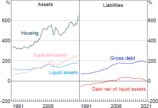
As has been well documented, household wealth has increased relative to income over recent decades and both sides of the household balance sheet (assets and liabilities) have expanded (Ellis 2006; Piketty and Zucman 2014) (Figure 1). It is also well known that interest rates have been on a trend decline over recent decades (Mian, Straub and Sufi 2021), and that this decline in interest rates has contributed to higher housing prices and debt (Debelle 2004; Ellis 2005; Schularick and Taylor 2012; Jordà, Schularick and Taylor 2014). It is common in the mainstream media, and even among academic research, to read that higher housing prices and debt over recent decades has made the economy more financially fragile (Bartscher et al 2020).
Sources: ABS; Authors' calculations
But it is less well known that, as part of this process of balance sheet expansion, the value of household liquid assets (which includes cash, deposits, equities and bonds) has also risen rapidly relative to incomes. In other words, households have larger liquidity buffers today than in the past, which has helped to service the higher debt. When measured net of liquid assets, the trend rise in the household debt-to-income ratio in Australia has been much less significant over recent decades and, in fact, has been falling since the global financial crisis (Figure 1). Moreover, the value of household liquid assets now basically matches the value of gross household debt, at least at an aggregate level.
We argue that the rise in household liquidity is a ‘side effect’ of the growth in housing prices and debt and the trend decline in interest rates over recent decades. In a world of uncertainty, many home owners with mortgage debt value liquidity for precautionary reasons, given the potential for future income or consumption falls. Rising levels of mortgage debt (relative to incomes) make mortgage payments larger and the risk associated with any income shock also increases. Households have responded to this increased risk by saving more for precautionary reasons (Boar, Gorea and Midrigan forthcoming). The higher rate of saving has occurred through both amortising mortgage debt (including paying ahead of schedule) and saving in other liquid assets, such as bank deposits and equities.
Some of the same underlying forces that have contributed to the rise in housing wealth, such as the trend decline in interest rates, have also allowed households to build liquidity buffers by increasing the capacity to pay down existing levels of debt. The capacity to save through debt amortisation has been further supported by mortgage market innovations, such as offset and redraw accounts, which are common in Australia but unusual by international standards. These products make it easier and more cost-effective for home owners to save by paying down mortgage debt ahead of schedule. By rebalancing their wealth portfolios through debt amortisation, home owners can liquidate some of their housing wealth and therefore better smooth consumption. Overall, these developments in the mortgage market have contributed to reducing financial fragility.
To support this story, we undertake a detailed exploration of the determinants of household liquidity in Australia, in terms of both the distribution across households as well as over time. This exploration exploits a wide range of data sources, including national accounts, household surveys and loan-level data.
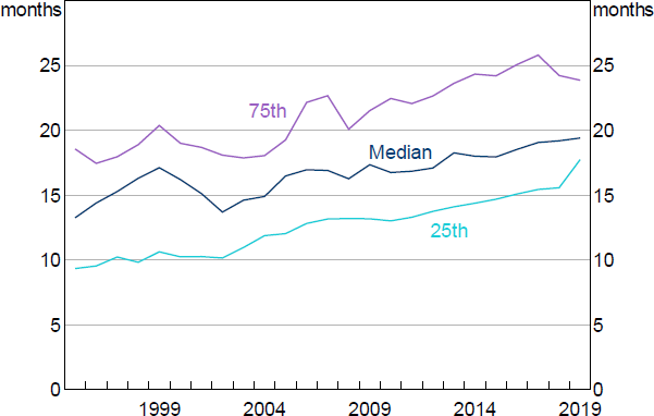
First, we document some facts about the cross-section and dynamics of household liquidity. For example, the average household holds a relatively large share of their asset portfolio in liquid assets. Household liquidity is unevenly distributed across the population, and this cross-sectional distribution is strongly correlated with the housing life cycle – specifically, age and housing tenure. Liquidity buffers have risen significantly relative to both income and spending since the start of the 21st century. The increase in liquidity in Australia has been broad based across the population, such that the share of liquidity-constrained households (with particularly low buffers) has gradually fallen over time. The decline in liquidity constraints has been strong among households with mortgage debt, even taking into consideration that households hold debt for longer now. The rise in household liquidity has not been specific to Australia but has been observed in basically all OECD economies since the start of the century (Figure 2).
Second, we provide evidence that the rise in household liquidity is closely linked to higher housing prices. The average household has not shifted the composition of their asset portfolios more towards liquid assets – instead, both liquid and illiquid wealth have risen relative to income. More specifically, households have responded to higher capital gains on housing, as well as increased mortgage debt, by increasing their holdings of liquid assets. Consistent with this, there is a strong positive correlation between the growth in housing prices and the growth in liquid assets across local housing markets in Australia, as well as across other advanced economies.
Sources: Authors' calculations; OECD
Third, we explore the mechanisms through which higher liquidity is linked to higher housing prices and debt. Consistent with the strong increase in liquidity buffers among home owners with mortgage debt (or ‘mortgagors’), most of the increase in aggregate household saving over the past decade is accounted for by mortgage debt amortisation. This is consistent with the idea that households often choose to accumulate wealth by saving in a ‘mortgage piggy bank’ (Bernstein and Koudijs 2021), possibly because housing provides a commitment device to reduce temptation and self-control problems (Attanasio, Kovacs and Moran 2021).
In Australia, paying down mortgage debt is a tax-effective method of saving for owner-occupiers. Principal payments on mortgage debt, including prepayments, explain almost all of the trend in the household saving rate over recent times (Figure 3). Home owners start with higher levels of debt today than in the past, but the rate at which debt is paid down has also risen. Saving in other assets has also been important during the COVID-19 pandemic.
We provide evidence that home owners facing greater income uncertainty, such as those worried about losing their jobs or that have more volatile incomes, hold relatively large liquidity buffers. Further, there is evidence that these households have increased their buffers by more than other indebted home owners. This suggests it is no coincidence that household liquid assets have grown alongside housing prices and debt. The rise in household liquidity is at least partly due to greater precautionary saving amongst owner-occupiers with mortgage debt.
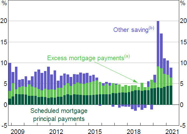
Notes:
(a) Sum of net flows into redraw and offset accounts
(b) Net of depreciation
Sources: ABS; APRA; Authors' calculations
But there are other causal mechanisms linking higher housing prices to higher liquidity. In an event study framework, we document that higher housing prices cause potential first home buyers to accumulate more liquid assets to finance housing deposits. This effect is stronger in recent years and in the more expensive capital cities of Sydney and Melbourne. This suggests that some of the growth in household liquid asset holdings is due to housing deposits increasing with housing prices. Higher housing prices can also support liquidity by increasing the capacity (and willingness) of home owners to withdraw equity and refinance their mortgages (Chen, Michaux and Roussanov 2020), and we find some empirical support for this too.
These mechanisms suggest that the rise in household liquidity is closely linked to the trend decline in interest rates that has been observed over recent decades in Australia and elsewhere. Specifically, disinflation and falling real interest rates have increased housing prices and housing deposits, and have also made it easier to amortise existing debt. This has boosted saving and allowed households with debt to accumulate wealth and build liquidity buffers. As further evidence, we use local projection methods to demonstrate that lower interest rates are associated with higher household liquidity buffers, including mortgage prepayment buffers, at the aggregate level.
Finally, we consider alternative explanations for the rise in household liquidity, including demand-side factors such as an ageing population and rising inequality, as well as supply-side factors such as changes in banking regulations. We find some evidence that the increase in liquidity is due to an ageing population and rising income inequality, although the effects are sensitive to the time period under consideration. We also find some evidence consistent with banks choosing to hold higher levels of deposits (as liquid liabilities) because of changes in bank liquidity regulations that were introduced following the global financial crisis.
There are two key motivations for our research. First, household liquidity buffers are important from a financial stability perspective. Past research has shown that the liquidity of household balance sheets is a key determinant of financial resilience. Households with limited buffers are typically more prone to financial stress. Low (or declining) liquidity buffers could pose a significant risk to financial stability, all other things being equal. Second, household liquidity buffers are important from a macroeconomic perspective. There is extensive research suggesting that household liquidity constraints are an important determinant of household spending (and its sensitivity to income and wealth shocks). But we know little about what determines household liquidity constraints.
There is a vast household finance literature that studies the determinants of household asset portfolios, and some of these studies look at the effect of housing on the household portfolio (e.g. Campbell and Viceira 2002; Curcuru et al 2010). However, these studies typically focus on housing price risk and the consumption commitment of housing as the underlying mechanisms (Chetty, Sándor and Szeidl 2017), and examine how housing investment and mortgage debt affects stock market participation (Flavin and Yamashita 2002; Cocco 2005). Overall, this literature typically focuses on the riskiness of the asset portfolio, such as low stock market participation, rather than the liquidity of that portfolio.[1] This is surprising given that liquid assets, such as bank deposits, typically comprise a much larger share of households' portfolios than risky financial assets, such as equities.[2]
To the best of our knowledge, we are the first to document the trend increase in household liquidity and its potential causes. Our empirical findings should therefore help in the development of new theoretical models to better understand why households hold such a high share of their wealth in liquid assets, and how household liquidity is linked to the housing market and the household's life cycle.
Our findings also have important policy implications from a financial stability perspective. First, the decline in liquidity constraints implies that the household sector may have become less sensitive to temporary income and wealth shocks, all other things being equal. Second, the decline in liquidity constraints, particularly among those with mortgage debt, has reduced the repayment risk associated with aggregate mortgage debt over the past couple of decades in Australia. Third, we show that housing equity is more of a liquid asset in Australia than in other countries due to financial innovations such as mortgage offset and redraw accounts. These financial products may mean that indebted households are less sensitive to income and wealth shocks in Australia than similar households in other countries. We leave this possibility to future research.
2. Institutional Features of the Australian Mortgage Market
Mortgage offset accounts and redraw facilities are features of the Australian mortgage market that are unusual by international standards. These accounts increase the liquidity of housing wealth and makes it easier for households to save through mortgage prepayment.
Mortgages with offset accounts currently comprise around 40 per cent of mortgages in Australia. An offset account is an at-call deposit account that is directly linked to the mortgage loan. Funds deposited into an offset account reduce the effective outstanding loan balance and therefore the interest payable on the loan. Mortgages with redraw facilities make up around 70 per cent of the total number of home mortgages in Australia.[3] A redraw facility enables the borrower to withdraw excess funds they have already contributed to pay off their loan. The balance of the facility consists of any extra payments the borrower has previously made towards paying their loan, above the amount required by the loan contract.
These mortgage products are a tax-effective method of saving. First, the effective deposit rate is the mortgage interest rate because the borrower ‘saves’ on interest payments by holding money in an offset account. Second, the account generates no tax compared to depositing money into a separate savings account where any interest accruing adds to taxable income. This means there can be large tax advantages for borrowers to pay off owner-occupied properties while still retaining access to the funds (mortgage interest payments are not tax deductible for owner-occupier loans, though they are for investor loans).
The main differences between offset accounts and redraw facilities are the degree of liquidity and the effect of withdrawals on home equity. In terms of liquidity, the funds sitting in an offset account are at call and easily accessible for withdrawal and for purchasing goods and services. The money in a redraw facility, while accessible, is not available for same-day, at-call withdrawal. The redraw has to be transferred to a deposit account before being spent. There may also be fees associated with redrawing money from the loan and limits on how often the redraw facility is used. Also, a withdrawal from an offset account does not affect the principal balance of the loan, whereas a redraw increases the principal and hence reduces the equity in the home. In other words, offset accounts are a type of deposit account linked to a home loan and the balances in offset accounts do not reduce the mortgage principal outstanding, but balances in redraw accounts do reduce credit outstanding.[4]
3. How Do We Measure Household Liquidity?
3.1 Data
In exploring the liquidity of household balance sheets we rely on a range of indicators, including aggregate national accounts data and various household surveys.
Aggregate household liquidity buffers are measured using national accounts data from the Australian Bureau of Statistics (ABS). The aggregate household liquidity buffer is the ratio of household liquid assets to disposable income. Household liquid assets is the sum of currency and deposits, bonds and equities in the financial accounts.[5] Household disposable income is gross disposable income and comes from the national accounts.
Our household-level data primarily come from the ABS Survey of Income and Housing (SIH) and the Household, Income and Labour Dynamics in Australia (HILDA) Survey. The SIH is a household survey that collects information on income, wealth, housing and various other household and personal characteristics. The SIH household-level data are available for biennial years from 2003/04 to 2017/18.[6] The SIH person-level data include characteristics such as labour force status, industry of work, hours worked and education. Since 2007/08, the SIH includes a loan-level module that contains characteristics of each loan, including the main purpose of a loan, amount borrowed, principal outstanding and year of loan origination. We use the Household Expenditure Survey (HES) collected by the ABS as a complement to the SIH. The HES and the SIH are run together every six years, and 2015/16 is the latest cycle of the joint surveys. Since 2003/04, the HES has also included a loan-level module, which allows us to explore loan-level data spanning two decades.
The HILDA Survey is an annual Australian survey that tracks a representative group of individuals (roughly 17,000 people from 9,000 households) between 2001 and 2019. Through personal interviews and self-completed questionnaires, the survey collects detailed information on households, including income and spending. Every four years the survey includes a wealth module, which collects detailed information on household assets and liabilities; the latest observation for household wealth is for 2018.
The ABS distributional accounts integrate micro (the SIH) and macro (national accounts) sources and produce distributional information of household income, consumption and wealth. This dataset is broadly representative of the Australian household sector and includes people living in non-private dwellings (such as nursing homes) and people in very remote communities, who are often out-of-scope in micro datasets. In this dataset, the relevant household information, such as age, is grouped according to a designated ‘household reference person’.[7] The distributional accounts divide household assets, debts and income into different income, wealth and age groups. This allows us to track how liquidity buffers evolve within each group. The time series are available for biennial years from 2003/04 to 2017/18. Household liquidity buffers are measured using the same method as the national accounts.
We also use banking data on household balance sheets. The Australian Prudential Regulation Authority (APRA) collects monthly statistics from authorised deposit-taking institutions, such as banks. This information includes the number and value of offset and redraw accounts, as well as household deposits, at each institution.
3.2 Definitions
3.2.1 Household liquidity buffers
Household liquidity buffers are measured as the ratio of household liquid assets to household disposable income. Here, household liquid assets includes cash, bank deposits, equities and bonds. Where possible, liquid assets also include mortgage offset and redraw accounts. The exact measurements vary in different household surveys depending on data availability. For the cross-sectional analysis in the 2017/18 SIH, we also consider an alternative measure in which superannuation balances are assumed to be fully liquid for retired households.
In the SIH, for households with mortgage debt, mortgage prepayments (offset and redraw accounts) are included in the measure of liquidity buffers where possible. Since 2011/12, the SIH has included information on the value of offset accounts, but we do not directly observe the balance of redraw accounts. Instead, we estimate redraw balances for amortising loans based on other information drawn from the SIH loan-level data. This includes the year of loan origination and the current (and initial) loan balance.[8] The relevant interest rate is derived from RBA statistical table ‘F5 Indicator Lending Rates’.
The scheduled payment is calculated using a standard loan amortisation formula that has a 30-year loan term and an interest rate equal to the average annual variable interest rate:
where D0 is the initial loan balance, i is the interest rate and n is the loan term.
The scheduled payment can then be split into the interest component by multiplying the interest rate by the outstanding loan balance and the principal component which is the residual.
The redraw balance is the difference between the estimated scheduled balance and the reported outstanding balance, where the scheduled balance ( Ds ) is calculated as:
where all the terms are as before, except for the inclusion of the remaining loan term ( k ). The derivation of these formulae can be found in Appendix A. The definition of liquid assets in the HILDA Survey does not include offset and redraw accounts because it is not possible to separate out the value of offset accounts from total deposits due to changes over time in the treatment of offsets in the survey.
3.2.2 Liquidity-constrained (or ‘hand-to-mouth’) households
We follow the framework of Kaplan, Violante and Weidner (2014) to estimate the share of households that are liquidity constrained, or hand-to-mouth. This is based on a two-period intertemporal consumption model in which households make two decisions: 1) how much of their income to save, and 2) how much to save in the form of liquid versus illiquid assets. The illiquid asset offers a higher return than the liquid asset, but there is a transaction cost associated with accessing it. Conceptually, households have two kinks in their budget constraints – one at zero liquid assets (a household can have negative liquid assets if they borrow, but this is costly), and one, if they do have access to credit, at their credit limit. Under certain parameters, some households will choose to save entirely through illiquid assets: that is, they optimally choose not to smooth through fluctuations in income, and instead keep only as much liquid wealth as they intend to consume in that period. In other words, constrained households optimally choose to consume at the kinks, implying that they will have a marginal propensity to consume out of income which is equal to unity.
In practice, identifying households that are at these kinks is a challenge. Ideally, we would observe each household at the end of their pay period in order to identify their outstanding level of liquid assets. But the annual surveys are snapshots at a single point in time (usually the date of the interview) that will not necessarily correspond to the end of the pay period. Moreover, even people who spend all of their income each pay period will spend it only gradually. So, at the time of the interview, some households that report having positive liquid assets (because they are in the middle of a pay period) will have zero liquid wealth by the end of the period. These households will be wrongly classified as not hand-to-mouth if we look only for households with liquid assets exactly at the budget constraint kinks at the time of the interview. Accordingly, the number of surveyed households that report having zero liquid assets (or negative liquid assets equal to their credit limit) is likely to underestimate the total number of hand-to-mouth households.
To partly account for this timing problem, we follow their methodology in assuming that households consume their liquid assets at a constant rate, and identify households as ‘hand-to-mouth’ (HtM) if:
- their liquid wealth balance is positive, but less than half their income each pay period; or
- their liquid wealth balance is negative, and is less than the difference between half their income each pay period and a credit limit.
We can also divide hand-to-mouth households into two groups:
- the wealthy hand-to-mouth, who have positive illiquid asset balances; and
- the poor hand-to-mouth, who have zero or negative net illiquid assets.
4. Stylised Facts about Household Liquidity
4.1 How is liquidity distributed across households?
We examine the cross-sectional distribution of household liquidity using household-level data from the 2017/18 SIH. The household-level module collects detailed information on households' income and wealth. For retirees, we assume their superannuation balances are fully liquid. We assume a person is retired if the person receives regular superannuation income.
The distribution of liquidity across households is strongly related to the housing life cycle – both in terms of age and housing tenure. Older households and outright home owners (that are typically retired) hold the highest shares of liquid assets relative to income. This is true whether we consider superannuation is fully liquid for retired households or not. In contrast, young households and renters typically hold the lowest liquidity buffers and are much more likely to be liquidity constrained.
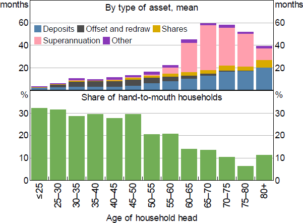
Household liquidity buffers tend to increase with the age of the household head (Figure 4). Similarly, the share of liquidity-constrained households falls significantly with age. This is consistent with the intuition that households gradually accumulate assets over their lifetimes and are more able (and willing) to diversify towards liquid assets, such as shares and bonds, as they get older.
Sources: ABS; Authors' calculations; RBA
Most young households (< 35 years) have a liquidity buffer of less than six months, with much of this stored in bank deposits. By middle age, people tend to move into home ownership and store much of their liquidity in redraw and offset accounts. When people reach retirement age, their liquid assets increase significantly as funds in their superannuation accounts become liquid. Even abstracting from superannuation balances, household liquid assets increase with age.
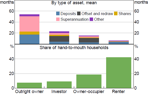
Liquidity is unevenly distributed across households with different housing tenure (Figure 5). Outright home owners have the largest liquidity buffers on average, partly because they are more likely to be retirees that can access superannuation but also because they no longer have the expense of a mortgage. Abstracting from superannuation balances, outright home owners still have larger buffers on average. In contrast, young renters typically hold the lowest shares of liquid assets and more than 40 per cent of renters are estimated to be liquidity constrained. Renters are typically younger and have had less time to build wealth.
Sources: ABS; Authors' calculations; RBA
Housing investors have the largest liquidity buffers among indebted households.[9] The average housing investor has a liquidity buffer of around two years' worth of income and is much less likely to be liquidity constrained than other households. Moreover, indebted investors that own multiple rental properties have even larger liquidity buffers on average. First home buyers have the lowest liquidity buffers among households with a mortgage, consistent with these households being at a relatively early stage in the life cycle. However, first home buyers are not more likely to be liquidity constrained than other indebted home owners. This may be because many first home buyers choose when to buy and how much to spend on a home, and hold just enough liquidity to keep them out of financial trouble after their purchase decision. Alternatively, lenders may be more likely to lend to borrowers that have a relatively large buffer after taking on mortgage debt.
To more closely examine the cross-sectional determinants of household liquidity buffers a simple regression was estimated based on the household survey data. The regression results support the graphical findings. In particular, factors associated with the housing life cycle, such as age and housing tenure, are important determinants of the distribution of buffers across households.
4.2 How has household liquidity changed over time?
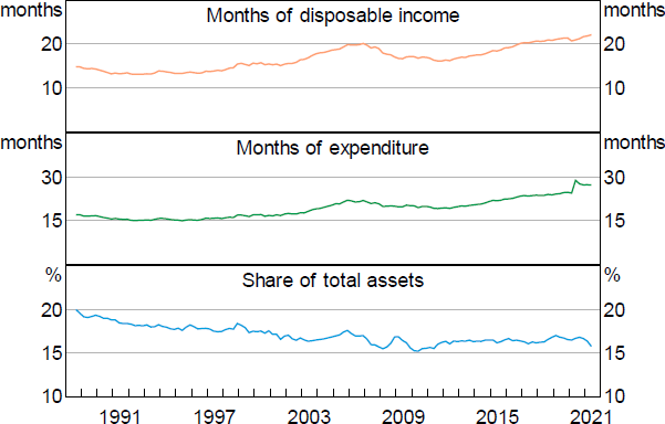
Turning to the dynamics of household liquidity, we find that household liquidity buffers have risen strongly over the past couple of decades. This is true when measured against income (top panel of Figure 6) or spending (middle panel). But, importantly, the ratio of liquid assets to total assets has not changed much at all over the last two decades (bottom panel of Figure 6). This suggests that households have not shifted their asset portfolios more towards liquid assets. Instead, household balance sheets have expanded, with both liquid and illiquid assets rising relative to income. We find similar trends when looking across other OECD countries – see Appendix B.
Sources: ABS; Authors' calculations
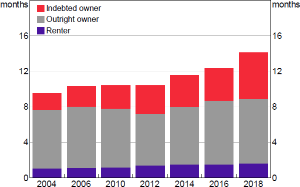
The increase in liquidity buffers is also apparent at the household level, with the average liquidity buffer steadily increasing since the early 2000s (Figure 7). The increase in liquidity is also very broad based across households, though housing tenure appears to be important in explaining the trend as well. Specifically, the rise in buffers has been largest amongst households with mortgage debt (Figure 8). For these households, higher buffers have been driven mainly by the increased value of offset and redraw accounts, which account for close to half their liquid assets.
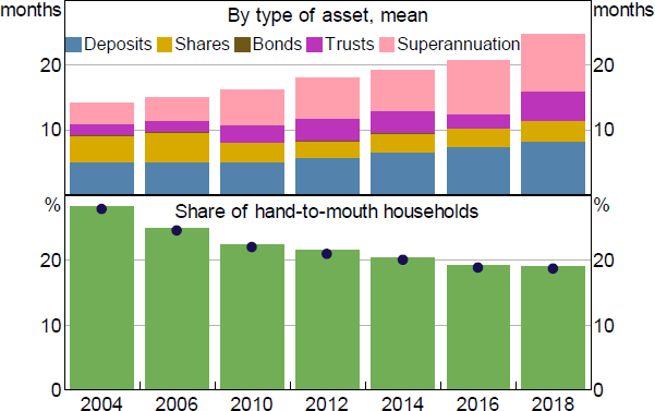
Notes: Deposits include offset accounts; dots represent share of hand-to-mouth households after adjusting for ‘liquid’ superannuation
Sources: ABS; Authors' calculations
Sources: ABS; Authors' calculations
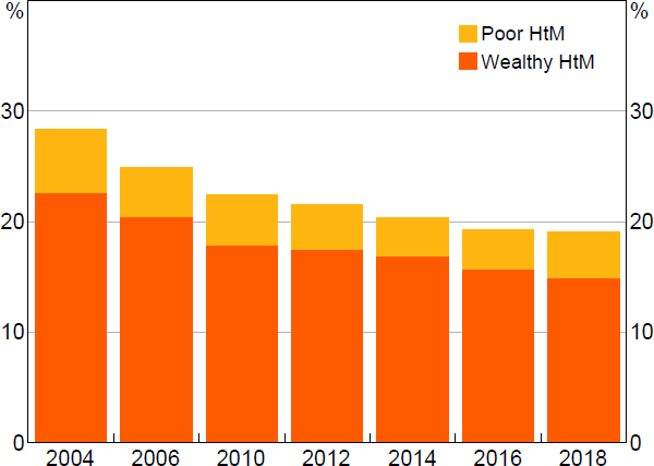
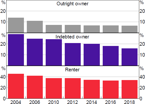
Consistent with the increase in average liquidity buffers, the share of liquidity-constrained households has generally fallen over the past two decades. Almost all of this decline in liquidity-constrained households is due to fewer ‘wealthy’ hand-to-mouth households, with the share of ‘poor’ hand-to-mouth households being broadly stable (Figure 9). The decline in the prevalence of liquidity constraints is broad based across age and housing tenure (Figure 10).
Sources: ABS; Authors' calculations
Sources: ABS; Authors' calculations
The introduction of mortgage offset and redraw facilities is likely to have increased the liquidity of housing wealth and contributed to the rise in aggregate household liquidity. At an aggregate level, around one-fifth of the increase in liquid assets (relative to disposable income) since the 2010s has been channelled into offset and redraw accounts. Among those with mortgage debt, increased wealth held in offset and redraw facilities accounts for about two-thirds of the increase in liquidity over the same period.
It is challenging to identify the causal effect of these innovations on liquidity buffers. This is because borrowers that select mortgages with such features could be systematically different from those that do not, and these systematic differences could reflect a range of borrower characteristics, some of which are likely to be unobservable (e.g. risk preferences). However, we can partly gauge the importance of offset accounts by separating borrowers into those that report having an offset account and those that report they do not, and controlling for a wide range of observed characteristics that are likely to be correlated with the decision to select such mortgages.
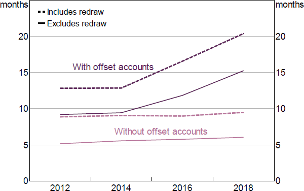
The increase in buffers amongst households with mortgage debt is mainly driven by households with offset accounts, at least since the 2010s (Figure 11).[10] Households with an offset account have larger buffers than those without offset accounts, on average. More notably, these households also experience a much larger increase in buffer, even after controlling for a range of household characteristics such as income, age and household size. This suggests that such innovations in the mortgage market have supported the rise in household liquidity.
Sources: ABS; Authors' calculations; RBA
4.3 How has household liquidity changed over the life of a loan?
Next, we examine how debt, repayments and liquidity evolve over the life of a mortgage using loan-level data drawn from the SIH and the HES that cover the period since 2003/04 at roughly two-year intervals.
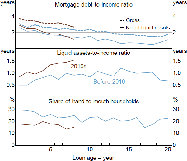
Not surprisingly, gross mortgage debt gradually falls relative to income as the loan ages and the debt is repaid (top panel of Figure 12). At the same time, liquid assets rise relative to income (middle panel of Figure 12), indicating that net debt (gross debt less liquid assets) falls even faster. Consistent with this, the probability of being liquidity constrained decreases with loan age (bottom panel of Figure 12), suggesting that borrowers become more resilient to balance sheet shocks as loans age, all else equal.
Sources: ABS; Authors' calculations; RBA
The life cycle evolution of debt can also be estimated for different ‘birth cohorts’ of mortgages. For this, mortgages are split into two groups – those loans originated before and after 2010. In the early years of loan life, the gross debt-to-income ratio is slightly higher on loans originated in the 2010s compared to those originated earlier, consistent with a higher housing price-to-income ratio at birth. However, the net debt-to-income ratios are similar for the two birth cohorts, indicating that liquidity buffers are larger (and growing more quickly) for the more recent cohort. Similarly, borrowers with loans originated in the 2010s are much less likely to be liquidity constrained than earlier loan cohorts.[11]
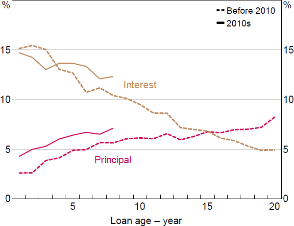
The loan-level information also allows us to split scheduled mortgage payments into interest and principal payments over the loan life cycle. Consistent with the function of a credit foncier model, we observe a steady decline in the share of income going to interest payments and an offsetting increase in the share going to principal payments as the loan ages (Figure 13). Clearly, the ratio of principal payments to income is much higher for loans born in the 2010s than for earlier birth cohorts. This is consistent with borrowers being able to build buffers more quickly in the 2010s compared to earlier decades, and provides a saving mechanism through which mortgagors can build liquidity.
Sources: ABS; Authors' calculations; RBA
5. Household Liquidity and Mortgage Debt Dynamics
Taken together, the stylised facts indicate that there is a close link between the rise in household liquidity, the housing life cycle and the mortgage market. In this section, we outline the channels through which changes in household liquidity may be linked to changes in housing prices and debt.
To identify the channels through which mortgage debt, housing prices and household liquidity are related, we provide a conceptual framework based on a partial equilibrium two-period consumption model in Appendix D. Based on this framework, we outline each channel in turn and provide some testable predictions about the correlations between liquid assets, housing prices and mortgage debt which we take to the data:
- Housing deposit channel: households accumulate liquid assets for the deposit to purchase a home. This is typically around 10–20 per cent of the value of the home for a first home buyer. If this channel matters, we should observe a sharp decline in liquid assets at the time of first home purchase (as the buyer converts the liquid assets to housing equity). Assuming that housing prices continually rise, we should observe higher levels of liquidity prior to purchase over time and this effect should be particularly strong in more expensive housing markets, such as the large capital cities.
- Precautionary saving channel: home owners might increase their buffers for precautionary saving reasons, for example, because of increased uncertainty about future income or mortgage repayments. If precautionary saving matters, we should observe higher buffers for home owners that face greater income uncertainty, such as those that are more worried about losing their jobs or those that have more volatile incomes.
- Housing equity withdrawal channel: households can extract equity from their homes (at a cost) and this money can be consumed or saved in liquid assets, assuming they have positive home equity. A home owner can do this either by taking out a home equity loan or by selling their home and moving to a new home with less equity. Alternatively, home owners can refinance their mortgages to a lower interest rate to reduce the scheduled payment and free up money that can be consumed or saved in liquid assets. This channel predicts a positive correlation at the household level between the growth rate of debt and liquid assets at the time of equity extraction or refinancing.
5.1 The housing deposit channel
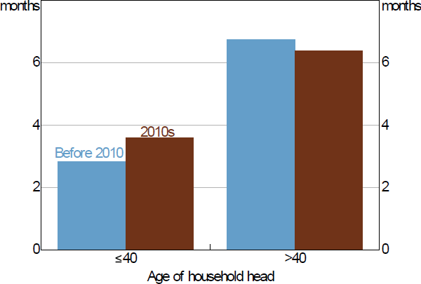
First, we consider whether the rise in household liquidity over time is connected to rising deposit requirements to purchase a home. If true, we should observe an increase in liquidity buffers among young renters – the households that are most likely to be potential first home buyers. We do find some evidence that buffers have increased among young renters (those with a household head aged less than or equal to 40 years) relative to older renters over the past decade (Figure 14).
But we can more closely identify the housing deposit channel by adopting an event study approach and examine what happens to liquidity when a household buys a home for the first time. For this, we need to track the liquidity position of a household before, during and after they purchase their first home, which requires longitudinal information from the HILDA Survey. We infer information on when each home owner bought their home, how much they paid for the home, and how much debt they took on at the time from the wealth modules (that are available every four years).[12]
Sources: ABS; Authors' calculations
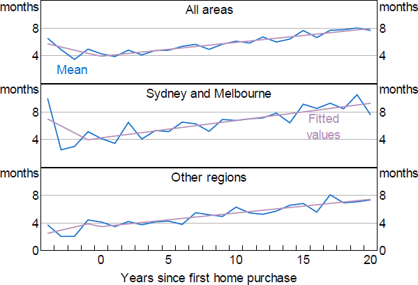
The event study indicates that, for those households that enter into home ownership, liquidity buffers are typically high in the years just prior to purchase, but drop sharply around the time of purchase, as the household converts their liquid savings to finance the deposit (Figure 15).[13] Following the purchase, the average new home owner gradually accumulates liquid wealth, but the level of buffer does not return to its pre-purchase level until at least 5 to 10 years after purchase.
The drop in liquidity at the time of first home purchase is also larger for households living in Sydney and Melbourne than elsewhere in the country. This is consistent with households in more expensive areas needing to save up more (or longer) for a deposit. Further, there are cohort effects in that first home buyers today start with higher levels of liquidity buffer prior to purchase than those first home buyers a decade ago. This suggests that rising housing prices have lifted the deposit requirement and this has played some role in explaining the trend increase in liquidity buffers.
Sources: Authors' calculations; HILDA Survey Release 19.0
5.2 The precautionary saving channel
In a world of uncertainty, indebted home owners may value liquidity for precautionary reasons, given the potential for future income falls or unexpected increases in interest rates. Rising levels of mortgage debt (relative to incomes) make the mortgage payments larger and the risk associated with any income or payment shock increases. Households may respond to this increased risk by increasing their rate of precautionary saving. The higher rate of saving can occur through both amortising mortgage debt (including paying ahead of schedule) and saving in other liquid assets, such as bank deposits and equities.
In this section, we examine the evidence that precautionary saving behaviour is important to explaining liquidity buffers amongst mortgagor households. For this, we construct two measures of household-level uncertainty.
First, we construct a forward-looking (subjective) measure based on the beliefs of working households about their future job prospects. The HILDA Survey directly asks workers for an estimate of the probability that they will lose their job in the year ahead. This subjective measure of job loss has been shown to have some predictive ability for actual job loss (Penrose and La Cava 2021). Workers are assumed to be more ‘uncertain’ the higher their subjective estimate of potential job loss is. This is referred to as the ‘forward-looking’ measure of income uncertainty. Workers that expect to lose their job are assumed to be more likely to engage in precautionary saving behaviour. We should therefore observe higher buffers among these households.
Second, a backward-looking (objective) measure is constructed based on the observed volatility of past household income. Households that have more volatile income streams are assumed to be more likely to save for precautionary reasons. The household-specific estimate of income volatility is constructed in a few steps. Household income is assumed to be a function of observable household-specific characteristics based on the following OLS regression model:
where the dependent variable is the log level of household disposable income ( yit ) and the determinants ( Xit ) include household-level characteristics such as a household head's age, education and whether they have a long-term health condition, as well as worker characteristics including job tenure, occupation, the nature of the labour contract (e.g. fixed or part-time basis) and the industry of work. From this regression model the residual income is estimated for each household and year . The standard deviation of this residual income is then constructed over rolling three-year windows to obtain an estimate of income volatility. This is referred to as a ‘backward-looking’ measure of income uncertainty.
To test whether precautionary saving matters, we estimate the following panel regression:
where the dependent variable is the level of liquidity buffer measured as the ratio of liquid assets to disposable income in each year ( BUFFERit ) and the key explanatory variable is an indicator for the extent to which each household is exposed to income uncertainty, which is based on either the forward-looking or backward-looking indicator ( UNCERTAINTYit ). We also include a set of control variables for borrower characteristics that matter to the accumulation of liquidity such as the age of the household head, the age of the loan, disposable income and the housing price-to-income ratio.
The regression results indicate that households facing higher income risk are more likely to have larger liquidity buffers, as shown by the positive coefficient on each of the income uncertainty indicators (Table 1). This is consistent with these households saving for precautionary reasons. Based on the forward-looking indicator, a 1 percentage point increase in the expected probability of job loss (i.e. from a mean of 10 per cent to 11 per cent) is associated with a mortgagor household holding an additional $13,000 in liquidity buffer (or 0.13 additional years of income), all other things being equal. Similarly for the backward-looking indicator, a one standard deviation increase in income volatility is associated with mortgagor households holding an additional $25,000 in liquidity buffer (or 0.25 additional years of income), all else equal.
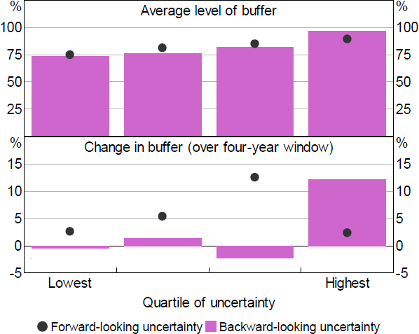
To examine the role of income uncertainty in explaining the trend in liquidity buffer over time, the income uncertainty indicators are split into quartiles based on the level of uncertainty.[14] The top (bottom) quartile includes the households facing the most (least) income risk (Figure 16). The HILDA Survey estimates generally indicate that liquidity buffers increased more between 2002 and 2018 for the households facing higher income risk. This is mostly true of the backward-looking indicator. This suggests that precautionary saving behaviour explains some of the increase in liquidity buffers amongst households with mortgage debt. However, the share of households facing higher income risk is not large enough to fully explain the rise in aggregate liquidity buffers, suggesting that other forces are at play too.
| Forward-looking indicator (working mortgagor households) |
Backward-looking indicator (all mortgagor households) |
|
|---|---|---|
| Income uncertainty | 0.13* (1.89) |
0.25*** (3.46) |
| Disposable income (log level) | 0.06 (1.27) |
0.04 (0.92) |
| Housing price-to-income ratio | 0.03*** (2.84) |
0.02*** (2.67) |
| Fixed effects | No | No |
| R squared | 4.7 | 4.5 |
| Households | 3,708 | 3,958 |
| Observations | 7,170 | 7,704 |
|
Notes: *, ** and *** denote statistical significance at the 10, 5 and 1 per cent levels, respectively; standard errors are clustered by household with t-statistics in parentheses; the regressions are also bootstrapped to address the generated regressor for the backward-looking uncertainty indicator; coefficient estimates for the constant and dummies for loan age, age of household head and survey year are omitted Sources: Authors' calculations; HILDA Survey Release 19.0 |
||
Notes: Buffer measured as the ratio of household liquid assets to disposable income; liquid assets include the value of cash, deposits, equities, bonds, trusts and estimated redraw balances
Sources: Authors' calculations; HILDA Survey Release 19.0
5.3 The housing equity withdrawal and refinancing channels
There was considerable product innovation in the Australian mortgage market through the late 1990s and the first half of the 2000s (Debelle 2010). Lenders introduced products such as home equity withdrawal loans and reverse mortgages, which allows households to borrow against the equity they have built up in their homes. Lenders also introduced interest-only loans and shared equity loans, which made it easier for households, particularly first home buyers, to purchase homes.
Since that time, housing equity withdrawal (HEW) has become relatively commonplace in Australia, with close to one in ten borrowers withdrawing equity from their home in any given year, according to estimates from the HILDA Survey. A 2006 survey of home owners also indicated that more than half of the equity withdrawn was used for asset accumulation, with deposits accounting for around one-third of all withdrawn funds (Schwartz et al 2006). This is consistent with households rebalancing their portfolios towards liquid assets in response to greater housing wealth.
To examine the effect of these mortgage products on household liquidity, we study the liquid asset accumulation of borrowers in the HILDA Survey. We can split borrowers into those that report either having a home equity loan or have refinanced since they took on a mortgage. If debt amortisation is associated with higher liquidity, we should observe a negative correlation between the growth rate of debt and liquid assets for a given borrower over time. But if the housing equity withdrawal/refinancing channel is important in practice, we should observe a weaker negative correlation between mortgage debt amortisation and liquid asset growth for households that extract equity or refinance. This is because mortgage debt and liquid assets simultaneously increase, at least temporarily, in these cases.
To test this hypothesis, we estimate the following panel regression:
where the dependent variable is the dollar change in liquid assets each ‘period’ and the explanatory variables include the dollar change in mortgage debt , a dummy for whether the borrower reports refinancing or withdrawing equity within the current period ( HEWit ) and an interaction between that dummy and the change in mortgage debt . We also include a set of control variables for borrower characteristics that could matter to the accumulation of liquidity such as age, income and the growth rate of housing prices, as well as lagged levels of both liquid assets and mortgage debt. Note that by taking differences in balance sheet positions over time we also implicitly control for borrower characteristics that do not vary over time but could matter to the level of household liquidity, such as risk preferences or financial literacy.
As the full balance sheet of households is only reported every four years in the HILDA Survey, a ‘period’ here refers to a four-year window. As such, a borrower is reported to have refinanced or withdrawn equity if they report doing so at any time within the past four years. As the effect of equity withdrawal or refinancing on liquid asset accumulation is likely to be temporary (and perhaps only captured within a year of refinancing) the estimation of the regression using four-year windows may attenuate the estimates and make it more difficult to identify such a channel.
The regression estimates indicate that each dollar of mortgage amortisation is associated with an increase of around 8 to 10 cents in liquid assets, on average (Table 2, first row). This is consistent with mortgage debt amortisation being associated with an increase in the value of liquid assets. More importantly, the debt amortisation effect is weaker for loans that have either been refinanced or have been used for HEW (Table 2, second row). This is consistent with the process of HEW or refinancing being associated with temporary increases in both debt and liquidity. This provides evidence that households rebalance their wealth portfolios in response to higher housing prices by building more liquidity through such channels.[15]
| OLS | |||
|---|---|---|---|
| No controls | With controls | With interactions and controls | |
| Change in mortgage debt | −0.08*** (−7.69) |
−0.10*** (−7.67) |
−0.12*** (−7.47) |
| HEW * Change in mortgage debt | 0.05* (1.94) |
||
| Change in household disposable income | 0.24*** (3.75) |
0.24*** (3.74) |
|
| Change in housing prices | 0.07*** (5.17) |
0.07*** (4.92) |
|
| Fixed effects | No | No | No |
| R squared | 0.7 | 3.9 | 4.0 |
| Observations | 12,222 | 12,222 | 12,222 |
|
Notes: *, ** and *** denote statistical significance at the 10, 5 and 1 per cent levels, respectively; standard errors are clustered by household with t-statistics in parentheses; coefficient estimates for the constant and dummies for HEW, loan age, age of household head and year are all omitted; the sample period is every four years between 2002 and 2018 Sources: Authors' calculations; HILDA Survey Release 19.0 |
|||
6. The Rise in Household Liquidity and Falling Interest Rates
Next, we consider how the rise in household liquidity and mortgage debt is linked to the trend decline in interest rates that has been observed over recent decades in Australia and elsewhere. Identifying the effects of interest rates on the liquidity of household balance sheets is challenging. This is because lower interest rates can have both direct and indirect effects on aggregate household liquidity and mortgage debt, and these effects work in opposite directions. First, lower interest rates can contribute to higher housing prices and debt relative to incomes. This increases the value of illiquid assets on household balance sheets, particularly for home buyers that have taken on new loans. In this case, lower interest rates increase mortgage debt inflows. But lower interest rates also make it easier to repay existing debts through prepayments, thereby increasing mortgage debt outflows. The net effect on the change in the stock of mortgage debt (relative to income) depends on which effect dominates.
6.1 The effect of interest rates on aggregate liquidity and mortgage debt
We first study the effects of changes in interest rates on aggregate mortgage debt and household liquidity buffers. For this, we estimate a series of impulse response functions (IRFs) using the local projections (LP) method of Jordà (2005).[16] For each forecast horizon ( h ) we run a regression of the quarterly (cumulative) change in liquidity buffer on unexpected changes in the cash rate, or monetary policy ‘shocks’ (as measured by Beckers (2020)) ( mp ),[17] as well as controls for the lagged value of the buffer:
The impulse response of the cumulative change in liquidity buffer to the monetary policy shock is traced out by the estimates of the . For example, when h = 10, the left-hand side variable is the difference in the liquid asset-to-income ratio at quarter 10 and the liquid asset-to-income ratio at the time of the monetary policy shock (at quarter 0). The sample covers the period from 1994:Q1 to 2019:Q3 due to sample coverage of the monetary policy shock series.
The impulse response estimates indicate that the effect of a temporary monetary policy shock on household liquidity peaks between five to eight quarters after the shock, with the effect gradually fading beyond eight quarters (Figure 17). These effects are statistically significant. However, the economic magnitude is relatively small with an unexpected 1 percentage point reduction in the cash rate being associated with aggregate liquidity buffers rising by about 0.3 months of income at the peak. We also find that this effect comes through a combination of increases in both the value of bank deposits and equities in response to temporarily lower interest rates.
To isolate the effect of interest rates on liquidity through the housing market we repeat the same exercise and estimate IRFs for the effect of interest rate shocks on mortgage debt, including both the inflows (new loans) and outflows (prepayments). This allows us to explore the direct and indirect effects of interest rates on liquid assets through the housing market.
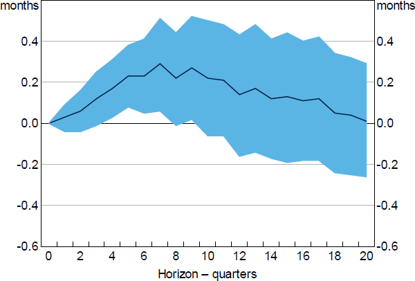
Note: Shaded area represents confidence interval based on +/– 2 standard errors
Sources: ABS; APRA; Authors' calculations
For this exercise, we measure mortgage inflows based on the value of new mortgage loans, excluding refinancing, each quarter as reported by the ABS. We then measure mortgage outflows as the residual difference between inflows and the change in the stock of mortgage debt. The inflows, outflows and the stock of mortgage debt are each scaled by household disposable income. The time window is restricted to the period between 2002:Q1 to 2019:Q3 as the ABS estimates of new lending begin at this time. The lack of business cycle fluctuations makes it harder to cleanly identify the effects of interest rates.[18]
An unexpected 100 basis point reduction in the cash rate is associated with an increase in new loans (relative to income) of 1 per cent after three to four quarters (Figure 18). The effect persists for about two years. This indicates that lower interest rates support new borrowing and the value of (illiquid) housing assets. But lower interest rates are also associated with a higher share of income going to prepayments. An unexpected 100 basis point cut in the cash rate is associated with mortgage debt outflows rising by about half a percentage point after six months. This is consistent with lower interest rates increasing the rate of debt amortisation and helping those with existing debt to build liquidity buffers. However, the effect is a bit more temporary than that on new lending. Overall, because lower interest rates boost both inflows and outflows, the net effect on the stock of mortgage debt is small. These interest rate effects on inflows and outflows remain, although are slightly weaker, when the regression includes controls for housing price growth over the forecast horizon. This suggests that the interest sensitivity of mortgage debt is partly explained by changes in housing prices.[19]
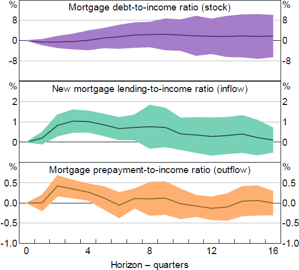
Note: Shaded area represents confidence interval based on +/- 2 standard errors
Sources: ABS; APRA; Authors' calculations
6.2 The effect of interest rates on household-level liquidity
The preceding analysis indicates that lower interest rates are associated with higher levels of mortgage debt and liquidity. We now look for causal links between interest rates, debt amortisation and liquidity buffers at the household level.
We test the hypothesis that mortgage borrowers that have experienced larger (cumulative) declines in interest rates over the life of the loan accumulate more liquidity buffer. For this, we rely on loan-level data from the SIH which provides estimates of both buffers and interest rates for each borrower and loan. However, the survey is a repeated cross-section and does not have a time dimension so we cannot track borrowers and loans over time. To introduce a time element, we rely on the fact that we can observe when the loan originated and we know the level of interest rates at that time, so we can approximate how much interest rates have changed over the life of the loan.
Consider a stylised example. There are two borrowers of the same age, income and housing wealth. Their loans are also very similar in that they originally borrowed the same amount of money, their loans are of the same age and they both currently face the same interest rate. However, the first borrower took out the loan when interest rates were higher than the other borrower. These ‘loan birth cohort effects’ will imply that the first borrower has experienced a larger unexpected decline in interest rates over the life of the loan compared to the second borrower. The first borrower should therefore have accumulated more buffer.
To formally test this, we specify the regression model as follows:
where the dependent variable is the level of the prepayment buffer ( PBUFFERit ) on loan i at survey year t. The prepayment buffer is measured as the difference between the scheduled balance and the outstanding balance divided by the level of household disposable income. The key explanatory variable is the cumulative change in interest rates since the start of the loan . This is measured as the difference between the current reported interest rate on the loan ( iit ) and the standard indicator rate for variable rate mortgages in the year of loan origination ( it–h ) for a loan of age h. The regression also includes controls ( CONTROLSit ) for borrower and loan characteristics, including: the (log) level of income, the housing price-to-income ratio and a full set of dummies for the age of the loan as well as the age group of the household head.
The results from the SIH loan-level data indicate that a 1 percentage point cumulative decline in interest rates is associated with an increase in prepayment buffer of around 0.82 per cent of household income (Table 3). This is true after controlling for a range of household and loan-level characteristics.
The regression estimates may be affected by endogeneity if, for example, interest rates are predictably lower during recessions, and borrowers choose to enter the market during these times to take advantage of such lower rates. To account for this borrower selection effect, we also estimate the model controlling for loan birth cohort effects, by including dummies for each year of loan origination (and dropping the year fixed effects). In this specification, the coefficient on the cumulative interest rate captures the difference in buffer between two loans, both born at the same time, but where one has experienced a larger decline in interest rates. In this case, the estimated effect of interest rates is stronger with a 100 basis point decline in lending rates being associated with buffers increasing by 1.12 per cent of annual income, all else equal.[20]
| OLS | ||
|---|---|---|
| No controls for birth cohorts | Controls for birth cohorts | |
| Cumulative change in interest rate | −0.82*** (−2.73) |
−1.19*** (−2.97) |
| Disposable income (log level) | −0.13*** (−7.25) |
−0.14*** (−7.36) |
| Housing price-to-income ratio | −0.00*** (−3.49) |
−0.00*** (−3.44) |
| Borrower fixed effects | No | No |
| Time fixed effects | Yes | No |
| Loan age fixed effects | Yes | Yes |
| Loan birth cohort effects | No | Yes |
| R squared | 3.7 | 3.7 |
| Observations | 28,361 | 28,361 |
|
Notes: *, ** and *** denote statistical significance at the 10, 5 and 1 per cent levels, respectively; standard errors are clustered by loan birth cohort, with t-statistics in parentheses; coefficient estimates for the constant and dummies for loan age, loan birth cohort, age group of household head and survey year are omitted; the sample period covers the survey years: 2003/04, 2007/08, 2011/12, 2013/14, 2015/16 and 2017/18 Sources: ABS; Authors' calculations |
||
Overall, the household-level regression results support the aggregate LP estimates and suggest that lower interest rates are associated with higher rates of saving and increased prepayment buffers for mortgagor households.
7. Alternative Explanations for the Rise in Household Liquidity
Based on the analysis in the preceding sections, the increase in household liquidity appears to be closely connected to the housing market. In this section we consider some other demand-side and supply-side factors that could explain the rise in household liquidity over recent decades.
7.1 Ageing population
An obvious demand-side explanation for the rise in household cash is an ageing population. Older households typically hold more of their portfolios in liquid assets and so an increase in the share of older households will mechanically increase the ratio of liquid assets to income in aggregate.
We find some evidence for an ageing population story using the distributional accounts. These accounts allow us to track how liquidity evolves both within and between different age groups in the economy. Between 2003/04 and 2017/18, the aggregate liquidity buffer rose by about 2½ months of disposable income. The distributional accounts indicate that the population aged 65 and above accounted for about one month of this aggregate increase (Figure 19).[21]
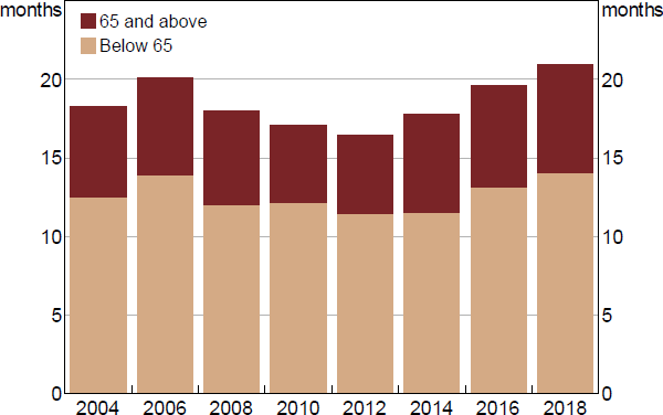
Sources: ABS; Authors' calculations
7.2 Higher income and wealth inequality
Along with an ageing population, we have observed an increase in both income and wealth inequality in Australia over the past two decades. If richer households hold a greater share of their portfolios in liquid assets then this rise in the concentration of income and wealth could also explain the rise in aggregate liquidity buffers. Based on the distributional accounts, richer households (in the top quintile) hold more of their wealth in liquid assets than other households (on either an income or wealth basis). Between 2003/04 and 2017/18 the top income quintile accounted for more than one month of the total increase of liquidity (of 2½ months of income) (Figure 20). This suggests that the rise in income inequality has been important to the rise in aggregate liquidity. However, the contribution of the top income quintile to the increase in aggregate buffer is sensitive to the sample period.
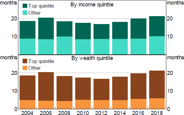
Sources: ABS; Authors' calculations
7.3 Higher demand for deposit liabilities amongst banks
The rise in household liquidity could also be due to supply-side factors. Retail deposits are a stable source of funding. Banks have increased their retail deposit funding since the global financial crisis (GFC) as they seeking more stable funding. The introduction of new liquidity regulations – such as the Net Stable Funding Ratio requirement that came into force at the start of 2018 – has supported the banks' demand for stable funding over recent years. Moreover, we find that the growth in the deposit share of banks' funding since the GFC is stronger at banks that started with relatively low levels of deposit funding in the pre-GFC period. This is consistent with banks competing harder for deposits by offering more attractive transaction and saving accounts, particularly through paying higher interest rates on these accounts. Retail deposit rates increased sharply in the period immediately after the GFC, though they have steadily declined over the past decade (Black, Titkov and Wang 2020).
8. Conclusion
It is well documented that household wealth has risen significantly in recent decades and that the value of both household assets and debt has increased. We document a less well-known phenomenon that has occurred in almost every advanced economy: household liquid assets have risen strongly relative to income over the same period.
Household surveys indicate that liquidity buffers are strongly associated with life cycle factors, such as age and housing tenure. The increase in buffers over recent decades has been broad based across households, though strongest amongst households with mortgage debt. Consistent with this, the share of liquidity-constrained households has declined significantly.
The growth in liquidity buffers is closely connected to developments in the housing market through multiple channels. First, higher housing prices have encouraged potential home buyers to accumulate more liquid assets in the process of saving for a deposit. Second, higher mortgage debt has increased the repayment risks associated with future income shocks and led indebted home owners to build liquidity buffers for precautionary reasons. The process of debt amortisation has been supported in Australia by unique financial innovations such as mortgage offset and redraw accounts that have increased the liquidity of housing wealth.
Our findings demonstrate that the decades-long expansion of household balance sheets does not necessarily mean that households have become overextended. A little recognised ‘side effect’ of rising housing prices and debt has been the increased rate of housing-related saving through higher mortgage principal payments. This increase in housing-related saving has been supported by the decline in interest rates and has allowed indebted households to build larger liquidity buffers. To the extent that more liquidity is associated with less financial stress, our results suggest that the higher ratio of debt to income has not made the household sector more financially fragile.
The significant decline in liquidity constraints amongst households with mortgage debt indicates that the repayment risk associated with aggregate mortgage debt has declined over recent decades. However, to the extent that rising housing debt has increased the risks associated with future income shocks, and hence caused households to reduce their spending for precautionary reasons, it may be welfare reducing from a macroeconomic perspective.
Finally, it is surprising how unique mortgage offset and redraw accounts are by international standards given their importance to the process of debt amortisation and the accumulation of liquidity buffers. These accounts make housing much more liquid and potentially allow home owners to better smooth consumption in the face of unexpected income and wealth shocks. It would be interesting to investigate the macroeconomic and financial stability implications of such mortgage accounts. For example, these accounts may make aggregate consumption less volatile in Australia than other comparable countries. They may have also reduced liquidity constraints by more in Australia than elsewhere, with a potential bearing on financial stability risks stemming from the household sector.
Appendix A : Derivation of the Loan Amortisation Formulae
The loan amortisation formulae for the outstanding debt balance and scheduled payment can be derived in a series of steps. For an amortisation schedule, define the function D ( t ), which represents the principal amount outstanding at period t. A formula for the principal amount outstanding in any given period can be derived given a scheduled payment ( m ) and contracted nominal interest rate (R = (1 + i)).
This process generalises to the principal amount outstanding in period t:
Given a geometric progression for the sum of the interest rate terms, this can also be written as:
Assuming that the loan is fully repaid after n periods, the outstanding balance will be completely paid off in the last payment period, which gives:
Solving for the scheduled payment ( m ) gives:
After substituting for the scheduled payment and simplifying, the outstanding balance in period t is:
Appendix B : Cross-country Evidence on Liquidity Buffers
To explore the cross-country determinants of household liquidity buffers we estimate a simple reduced-form regression model. The model is based on an unbalanced panel with 37 OECD countries and a sample covering the period from 1995 to 2019 (with more than 25 observations in each year):
where the dependent variable is the annual change in the ratio of household liquid assets to disposable income and the explanatory variables include the change in real interest rates, the change in the housing price-to-income ratio, the change in the mortgage debt-to-income ratio, population growth and consumer price inflation. The model is specified in changes to ensure stationarity (given a relatively long time series) and to remove any country fixed effects (that capture country-specific factors such as cultural and institutional differences that might explain the level of liquidity buffer). Liquid assets include currency and deposits, securities, shares and other equity. Long-term interest rates are based on government bonds maturing in ten years.
The regression estimates indicate that changes in liquidity buffers are correlated with both changes in housing prices and mortgage debt (relative to income)(Table B1). These results also suggest that countries with ageing populations are more likely to have higher buffers, which is consistent with older households holding more wealth in liquid assets). We also find that lower interest rates are associated with higher liquidity buffers, though the effect is economically small.
| Control for: | ||
|---|---|---|
| housing prices | mortgage debt | |
| Change in housing price-to-income ratio | 0.48*** (0.14) |
|
| Change in debt-to-income ratio | 0.46*** (0.12) |
|
| Change in inflation rate | −0.00 (0.00) |
−0.00 (0.00) |
| Change in real long-term interest rate | −0.00 (0.00) |
−0.00*** (0.00) |
| Population growth rate | 0.02 (0.62) |
0.07 (0.43) |
| Change in employment rate | −0.17** (0.06) |
−0.13* (0.07) |
| Change in share of population aged 65 and over | 0.61* (0.32) |
0.63** (0.27) |
| Constant | −0.01 (0.01) |
−0.00 (0.01) |
| R squared | 0.23 | 0.08 |
| Observations | 188 | 322 |
|
Notes: *, ** and *** denote statistical significance at the 10, 5 and 1 per cent levels, respectively; t-statistics in parentheses Sources: Authors' calculations; Jordà, Schularick and Taylor (2017); OECD |
||
To more clearly explore the effect of changes in interest rates on buffers, we estimate IRFs using the LP method of (Jordà 2005):
Specifically, for each forecast horizon, h, we run a regression of the household liquidity buffer on the long-term interest rate, as well as controls for the lagged value of the buffer, the change in the housing price-to-income ratio, the share of population aged 65 and above, GDP growth and consumer price inflation.
The results suggest that a decrease in the long-term interest rate of 1 percentage point is associated with a 3 per cent increase in the household liquidity buffer over a two to four year horizon (Figure B1). This is slightly larger than the estimated effect of interest rates on buffers for Australia.
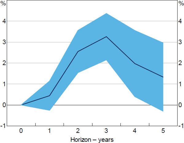
Note: Shaded area represents confidence interval based +/– 2 standard errors
Sources: Authors' calculations; Jordà, Schularick and Taylor (2017); OECD
Appendix C : Household Liquidity and Local Area Housing Prices
Consistent with the cross-country evidence, we also find that the increase in household liquid assets has closely matched the increase in housing prices across local housing markets. To see this, we divide the HILDA Survey sample into local housing markets based on the Statistical Area Level 4 (SA4). We estimate housing prices in each SA4 based on the average reported (subjective) estimate of housing prices by home owners in the survey.[22] There are about 107 SA4s in Australia and the population size of SA4s varies from around 40,000 to 900,000.
We explore the correlations between household liquidity buffers and both housing prices and mortgage debt (relative to income) across various regressions. The first regression estimates aggregate all liquid assets, housing wealth, mortgage debt and income by local housing market and year. We refer to these as the ‘weighted estimates’ because the ratios of liquidity, housing prices and mortgage debt to income are all aggregated over households, which implicitly puts more weight on richer households (Table C1). We can also estimate these regressions at the household level, but look at the correlation with aggregate local area housing prices, which we refer to as the ‘unweighted estimates’ (Table C2).
| Weighted estimates | Unweighted estimates | |
|---|---|---|
| Housing price-to-income ratio | 0.17*** (0.02) |
0.16*** (0.03) |
| Mortgage debt-to-income ratio | −0.32** (0.14) |
|
| Log of disposable income | −0.14 (0.16) |
|
| Constant | 0.43*** (0.09) |
2.55 (2.49) |
| Local area fixed effects | No | Yes |
| Year fixed effects | Yes | Yes |
| R squared | 0.16 | 0.58 |
| Observations | 435 | 435 |
|
Notes: *, ** and *** denote statistical significance at the 10, 5 and 1 per cent levels, respectively; t-statistics in parentheses; estimates for local area and year fixed effects are omitted Sources: Authors' calculations; HILDA Survey Release 19.0 |
||
| Indebted owners | All households | ||||||
|---|---|---|---|---|---|---|---|
| OLS | Fixed effects | OLS | Fixed effects | ||||
| No controls | Controls | No controls | Controls | ||||
| Housing price-to-income ratio | 0.18*** (0.04) |
0.21*** (0.05) |
0.08*** (0.03) |
0.05*** (0.02) |
0.05*** (0.01) |
0.02* (0.01) |
|
| Age | −0.21* (0.12) |
0.29** (0.13) |
−0.35*** (0.07) |
0.73*** (0.09) |
|||
| Age squared | 0.00*** (0.00) |
−0.00 (0.00) |
0.01*** (0.00) |
−0.00 (0.00) |
|||
| Log of household disposable income | 3.06*** (0.44) |
−1.51*** (0.45) |
2.73*** (0.40) |
−8.12*** (0.53) |
|||
| Household size | −0.52*** (0.10) |
0.23 (0.16) |
−1.57*** (0.12) |
1.06*** (0.16) |
|||
| Got pregnant in past year | 0.38 (0.40) |
0.68 (0.57) |
0.48 (0.34) |
1.58*** (0.38) |
|||
| Got sick in past year | −0.27 (0.54) |
0.71 (0.51) |
−1.04* (0.58) |
0.00 (0.52) |
|||
| Illness of family member in past year | −0.25 (0.35) |
0.14 (0.39) |
1.26*** (0.48) |
0.20 (0.43) |
|||
| Retired in past year | 1.83 (1.67) |
−0.17 (1.63) |
−0.12 (1.30) |
3.55*** (1.11) |
|||
| Birth of new child in past year | 0.31 (0.47) |
−1.01* (0.52) |
1.31*** (0.39) |
−1.09** (0.46) |
|||
| Got married in past year | −1.97*** (0.32) |
−0.67 (0.51) |
−1.96*** (0.64) |
1.38** (0.68) |
|||
| Got separated in past year | 0.47 (0.92) |
−0.06 (0.85) |
−1.34*** (0.52) |
−0.91* (0.52) |
|||
| Constant | 4.02*** (0.31) |
−26.08*** (4.27) |
10.75** (4.59) |
12.32*** (0.26) |
−17.30*** (3.79) |
66.46*** (4.41) |
|
| Household fixed effects | No | No | Yes | No | No | Yes | |
| Year fixed effects | No | Yes | Yes | No | Yes | Yes | |
| R squared | 0.03 | 0.06 | 0.02 | 0.01 | 0.14 | 0.04 | |
| Observations | 12,000 | 12,000 | 12,000 | 40,294 | 40,294 | 40,294 | |
| Households | 5,508 | 14,265 | |||||
|
Notes: *, ** and *** denote statistical significance at the 10, 5 and 1 per cent levels, respectively; standard errors are clustered by household with t-statistics in parentheses; estimates for household and time fixed effects are omitted Sources: Authors' calculations; HILDA Survey Release 19.0 |
|||||||
The regression results for the weighted estimates indicate that liquidity buffers are positive associated with local area housing price-to-income ratios. We also find that buffers are negatively associated with mortgage debt-to-income ratios after controlling for housing prices. This is consistent with the process of debt amortisation increasing liquidity for households, even at an aggregate (local area) level.
The regression results for the unweighted estimates also indicate that the liquidity buffers of indebted home owners are positively associated with local area housing price-to-income ratios. Moreover, this effect is stronger than for other households, including outright home owners and renters. This is shown by a comparison of the estimates in the first row across indebted home owners (columns 1 to 3) and all households (columns 4 to 6). The correlation exists even when controlling for a wide range of household-level characteristics.
Taken together, the results are consistent with households looking to rebalance their wealth portfolios towards liquid assets in response to changes in housing prices, and that the process of debt amortisation helps to build liquidity buffers, even at an aggregate level.
Appendix D : Household Liquidity, Precautionary Saving and Borrowing Constraints
To provide a conceptual framework for the empirical analysis consider the following two-period consumption model. A representative household maximises lifetime utility subject to an intertemporal budget constraint as well as two borrowing and saving constraints. The model is partial equilibrium in nature in that it takes income, housing prices and interest rates as given. To keep things tractable, we abstract from realistic elements such as the life cycle and decisions regarding housing tenure. The household is born with a single asset ( A0 ), which can be thought of as housing equity, with some fixed fraction of this asset assumed to be initially liquid . The fraction of the asset that is liquid is exogenously given by a technology that allows households to tap the money held in the asset (such as mortgage redraw accounts). The household can choose to either consume or save the liquid fraction of the asset in the first period.
We assume households have log utility in a single consumption good:
where the discount factor is
The budget constraint in period 1 is:
where first period consumption ( c1 ) must be no greater than ‘cash on hand’ ( x1 ) which is the sum of the first period income endowment ( y1 ), any borrowing (negative saving) ( –s ) and some fraction of the initial value of the asset , where the price of the asset is P at the start of the first period and the real volume of the asset is fixed at its initial value ( A0 ). Cash on hand represents the resources available for consumption and saving to the household, after the realisation of first period income, and can be thought of as the value of liquid assets in the first period.
The budget constraint in period 2 is:
where the household can consume from its second period income endowment ( y2 ), any saving, including accumulated interest ( Rs ), and the remaining (illiquid fraction) of the value of the asset, which is equal to P1 at the start of the second period.
This implies an intertemporal budget constraint:
The household potentially faces a saving constraint:
This can be thought of as a deposit requirement in that the household must hold enough liquid assets to cover some share of the future value of the asset. (This is the flipside of a more standard loan-to-valuation constraint).
The household may also face a borrowing (or equity withdrawal) constraint. Because only a certain fraction of the asset is liquid in the first period, a household may choose to liquidate some of the future value of the asset (which is here known with certainty). We assume that the household is limited to borrow some fraction of any increase in the discounted value of the asset between period 1 and period 2.
We first consider the optimal saving decision of the unconstrained household. Substituting the intertemporal budget constraint into lifetime utility, we find the optimal level of saving:
Note that, due to a wealth effect, household saving is a negative function of any increase in the value of the asset (assuming a positive real interest rate and a positive initial value for the asset):
Note also that, if the asset is fully liquid in the first period , this wealth effect disappears.
We can also consider the optimal saving decision of the household that is constrained by the deposit requirement. This represents the problem facing a potential first home buyer. The saving constraint naturally leads to the prediction that higher future asset prices require greater saving now, and hence a positive correlation between the value of the asset and saving for potential home buyers.
Next, we look at the optimal saving of the household that is constrained in terms of borrowing against the future value of their asset through equity withdrawal. This represents the problem facing an owner-occupier that is currently liquidity constrained but has some positive housing equity. If the borrowing constraint is binding, then the optimal level of cash on hand is:
Here, higher asset prices are associated with more cash on hand which could be saved or consumed in the first period:
This implies that equity withdrawal provides a mechanism through which households choose to save in a liquid asset (though households may also choose to consume this equity).
Finally, we introduce uncertainty into the model to highlight the role of precautionary saving. This allows us to consider the problem of the owner-occupier that is worried about becoming liquidity constrained in the future if there is a negative wealth shock. For simplicity, suppose the only source of uncertainty is about the future price of the asset. And consider a mean-preserving spread of the future asset price:
where the future asset price consists of a constant mean ( P ) and a stochastic component . Assume that and For expositional purposes, also assume that In this case, the household in the first period faces the following decision:
The first line is the optimality condition when the borrowing constraint does not bind (so the household perfectly smooths consumption). The second line comes from the household budget constraint in period 1 when the borrowing constraint does bind. This condition can be rewritten in compound form:
Given that we have introduced uncertainty in the model, the future asset price enters the equation in expectation. Suppose that uncertainty about the future asset price increases. Very low realisations of the asset price become more likely, which reduces the household's future income. The borrowing constraint becomes more likely to bind. To avoid this, the household reduces consumption and increases saving in period 1. This precautionary saving effect will be larger for households that hold larger initial (volumes) of the asset.
In effect, when there is uncertainty about future income (e.g. because of increases in interest rates or falls in income), an owner-occupier household may choose to save more today because they are worried about becoming liquidity constrained in the future.
References
Andersen AL, AS Jensen, N Johannesen, CT Kreiner, S Leth-Petersen and A Sheridan (2021), ‘How Do Households Respond to Job Loss? Lessons from Multiple High-Frequency Data Sets’, Centre for Economic Policy Research Discussion Paper DP16131.
Attanasio O, A Kovacs and P Moran (2021), ‘Temptation and Incentives to Wealth Accumulation’, NBER Working Paper No 28938.
Bartscher A, M Kuhn, M Schularick and U Steins (2020), ‘Modigliani Meets Minsky: Inequality, Debt, and Financial Fragility in America, 1950-2016’, Centre for Economic Policy Research Discussion Paper DP14667.
Baumol WJ (1952), ‘The Transactions Demand for Cash: An Inventory Theoretic Approach’, The Quarterly Journal of Economics, 66(4), pp 545–556.
Beckers B (2020), ‘Credit Spreads, Monetary Policy and the Price Puzzle’, RBA Research Discussion Paper No 2020-01.
Bernstein A and P Koudijs (2021), ‘The Mortgage Piggy Bank: Building Wealth through Amortization’, NBER Working Paper No 28574.
Black S, D Titkov and L Wang (2020), ‘Developments in Banks' Funding Costs and Lending Rates’, RBA Bulletin, March.
Boar C, D Gorea and V Midrigan (forthcoming), ‘Liquidity Constraints in the U.S. Housing Market’, The Review of Economic Studies.
Campbell JY and LM Viceira (2002), Strategic Asset Allocation: Portfolio Choice for Long-Term Investors, Clarendon Lectures in Economics, Oxford University Press, Oxford.
Chen H, M Michaux and N Roussanov (2020), ‘Houses as ATMs: Mortgage Refinancing and Macroeconomic Uncertainty’, The Journal of Finance, 75(1), pp 323–375.
Chetty R, L Sándor and A Szeidl (2017), ‘The Effect of Housing on Portfolio Choice’, The Journal of Finance, 72(3), pp 1171–1212.
Cocco JF (2005), ‘Portfolio Choice in the Presence of Housing’, The Review of Financial Studies, 18(2), pp 535–567.
Curcuru S, J Heaton, D Lucas and D Moore (2010), ‘Heterogeneity and Portfolio Choice: Theory and Evidence’, in Y Aït-Sahalia and LP Hansen (eds), Handbook of Financial Econometrics: Tools and Techniques, Vol 1, Handbooks in Finance, North-Holland, Amsterdam, pp 337–382.
Debelle G (2004), ‘Macroeconomic Implications of Rising Household Debt’, BIS Working Papers No 153.
Debelle G (2010), ‘The State of the Mortgage Market’, Address to Mortgage Innovation Conference, Sydney, 30 March.
Ellis L (2005), ‘Disinflation and the Dynamics of Mortgage Debt’, in Investigating the Relationship between the Financial and Real Economy, BIS Papers No 22, Bank for International Settlements, Basel, pp 5–20.
Ellis L (2006), ‘Housing and Housing Finance: The View from Australia and Beyond’, RBA Research Discussion Paper No 2006-12.
Flavin M and T Yamashita (2002), ‘Owner-Occupied Housing and the Composition of the Household Portfolio’, The American Economic Review, 92(1), pp 345–362.
Ganong P and P Noel (2018), ‘Liquidity vs. Wealth in Household Debt Obligations: Evidence from Housing Policy in the Great Recession’, NBER Working Paper No 24964.
Jordà Ò (2005), ‘Estimation and Inference of Impulse Responses by Local Projections’, The American Economic Review, 95(1), pp 161–182.
Jordà Ò, M Schularick and AM Taylor (2014), ‘The Great Mortgaging: Housing Finance, Crises, and Business Cycles’, NBER Working Paper No 20501.
Jordà Ò, M Schularick and AM Taylor (2017), ‘Macrofinancial History and the New Business Cycle Facts’, in M Eichenbaum and JA Parker (eds), NBER Macroeconomics Annual 2016, 31, University of Chicago Press, Chicago, pp 213–263.
Kaplan G, GL Violante and J Weidner (2014), ‘The Wealthy Hand-to-Mouth’, Brookings Papers on Economic Activity, Spring, pp 77–138.
Mian A, L Straub and A Sufi (2021), ‘What Explains the Decline in r*? Rising Income Inequality versus Demographic Shifts’, Becker Friedman Institute for Economics Working Paper No 2021-104.
Penrose G and G La Cava (2021), ‘Job Loss, Subjective Expectations and Household Spending’, RBA Research Discussion Paper No 2021-08.
Piketty T and G Zucman (2014), ‘Capital is Back: Wealth-Income Ratios in Rich Countries 1700–2010’, The Quarterly Journal of Economics, 129(3), pp 1255–1310.
Schularick M and AM Taylor (2012), ‘Credit Booms Gone Bust: Monetary Policy, Leverage Cycles, and Financial Crises, 1870–2008’, The American Economic Review, 102(2), pp 1029–1061.
Schwartz C, T Hampton, C Lewis and D Norman (2006), ‘A Survey of Housing Equity Withdrawal and Injection in Australia’, RBA Research Discussion Paper No 2006-08.
Simon J and T Stone (2017), ‘The Property Ladder after the Financial Crisis: The First Step Is a Stretch but Those Who Make It Are Doing OK’, RBA Research Discussion Paper No 2017-05.
Tobin J (1956), ‘The Interest-Elasticity of Transactions Demand for Cash’, The Review of Economics and Statistics, 38(3), pp 241–247.
Copyright and Disclaimer Notice
HILDA Survey Disclaimer
This paper uses unit record data from the Household, Income and Labour Dynamics in Australia (HILDA) Survey. The unit record data from the HILDA Survey was obtained from the Australian Data Archive, which is hosted by The Australian National University. The HILDA Survey was initiated and is funded by the Australian Government Department of Social Services (DSS) and is managed by the Melbourne Institute of Applied Economic and Social Research (Melbourne Institute). The findings and views based on the data, however, are those of the authors and should not be attributed to the Australian Government, DSS, the Melbourne Institute, the Australian Data Archive or The Australian National University and none of those entities bear any responsibility for the analysis or interpretation of the unit record data from the HILDA Survey provided by the authors.
Acknowledgements
We would like to thank Alex Ballantyne, Anthony Brassil, James Graham, Jonathan Kearns, Amanda Martz, David Norman, Isaac Pan, Matthew Read, Lars Svensson, Joyce Tan, Michelle Wright and seminar participants at the Reserve Bank of Australia, the University of Sydney-RBA Banking Reading Group Workshop and the Virtual Australian Macroeconomics Seminar for helpful comments and discussion. The views expressed in this paper are those of the authors and do not necessarily reflect the views of the Reserve Bank of Australia. The authors are solely responsible for any errors.
Footnotes
There is a closely connected, but older literature on household money demand that dates back to the models developed independently by Baumol (1952) and Tobin (1956). These models assume there is a trade-off between the liquidity provided by holding money (cash and deposits) to carry out transactions and the interest foregone by holding wealth in non-interest bearing assets. [1]
There is also a large literature that studies the effect of liquidity on asset prices, though much of the work focuses on the cross-section of company stock prices (and explains why some stocks are more liquid than others). [2]
Some mortgages have both an offset and redraw facilityso these proportions are overlapping andsum to more than 100 per cent. [3]
Another difference is the tax treatment of redraw accounts for investors compared to owner-occupiers. Investors with redrawaccounts cannot claim tax deductions on any withdrawn funds. [4]
Less than a fifth of bank household deposits are term deposits, which could be considered partly liquid, as they are able to be converted to cash only with advance notice and by paying a fee. We cannot directly identify term deposits in the household survey data. [5]
The 2007/08 SIH is omitted as some of the wealth variables were not collected. [6]
The household reference person is selected by the ABS based on a range of factors including home ownership status, income and age of the individuals within a household. [7]
The loan-level data required to estimate redraw balances are available in 2003/04, 2007/08 to 2017/18. [8]
Loan-level analysis of liquidity buffers for housing investors typically focus on prepayment buffers because they do not observe the entire balance sheet of the household. The full extent of the liquidity of investor balance sheets can only be observed in household surveys. [9]
Offset accounts data prior to 2010 are not available in the SIH. [10]
Further disaggregation of the liquidity buffers indicates that this difference in buffers between loan birth cohorts at the start of the loan is due to differences in deposit holdings, and particularly offset accounts. New borrowers may be choosing to take on more debt than required and saving some of the additional funds in offsets, as this increases liquidity without affecting the expected interest costs over the life of the loan. This is consistent with these innovations increasing the liquidity of housing wealth. [11]
We follow Simon and Stone (2017) to identify when households purchased their first home. [12]
The fitted values are estimated from a piecewise linear regression: Years since purchaseit * POSTit + Years since purchaseit * (1 – POSTit), where Years since purchaseit is the number of years since the home was purchased (which is negative for the years before purchase) and POSTit is a dummy variable which is equal to one if the year is after purchase and is zero otherwise. The underlying data on liquid assets is observed every four years in the survey. So, for example, a comparison of years 1 and 2 in the figure is a comparison of different households rather than the same household over time. This should be borne in mind when interpreting the trends in the figure. [13]
The distribution of the backward-looking uncertainty indicator is based on quartiles, while the distribution of the forward-looking indicator is based on terciles, with the bottom (low uncertainty) category including working households with an estimated subjective probability of zero job loss. [14]
An alternative way that home owners can extract home equity is by buying a home with less equity than their previous residence. We gauge the importance of this channel by studying the behaviour of liquidity buffers in the year of moving for moving home owners (treatment group) relative to moving renters (control group) within the same postcode. We find that home owners do increase their holdings of liquid assets during this period of moving, while the liquid asset holdings of renters remains relatively unchanged. This is again consistent with home owners choosing to rebalance their wealth portfolios in response to higher housing prices through a HEW channel. However, the effect appears to be concentrated amongst outright home owners. This channel therefore cannot explain the rise in liquidity buffers amongst households with mortgage debt. [15]
This is similar to the standard VAR approach but is less restrictive. However, the non-parametric nature of LP comes at an efficiency cost and may suffer from excessive variability. [16]
These ‘shocks’ capture changes in the cash rate that are not systematically related to changes in the RBA's forecasts for economic activity and inflation. [17]
The standard errors for the LP estimates are bootstrapped given that the monetary policy shock is a generated regressor. [18]
Further disaggregation of the mortgage debt outflows indicates that the effect of lower interest rates is due to both higher scheduled and unscheduled principal payments (relative to incomes). However, these estimates are based on a relatively short sample period since 2008, given this is when APRA began collecting the principal payments data. [19]
A further challenge to the identification strategy is that observed loan age is endogenous, being a function of the borrower's willingness and ability to refinance their mortgage. This propensity to refinance is likely to be a function of liquidity – with more constrained borrowers being more likely to refinance. However, this source of endogeneity works against finding a negative correlation between the change in interest rates and the size of the buffer. This is because a borrower with low buffer is more likely to refinance to a lower rate (and hence experience a larger cumulative decline) compared to a borrower with more buffer. This will induce a positive correlation between the level of buffer and the cumulative interest rate change. [20]
We find some role for the age structure of the population in predicting aggregate liquidity buffers based on the cross-country panel evidence in Appendix B. [21]
The HILDA Survey asks home owners to report the market value of their current home. The housing prices of renters are the average of the reported housing price of home owners in the area. [22]