Research Discussion Paper – RDP 2020-03 The Determinants of Mortgage Defaults in Australia – Evidence for the Double-trigger Hypothesis
1. Introduction
Mortgage defaults can have huge personal and financial stability costs. Understanding their determinants is important for understanding the risks associated with mortgage defaults, and how these can be mitigated. Yet there have been few studies of the determinants of mortgage defaults in Australia, likely reflecting relatively low default rates and the absence of widespread stress events for periods when detailed data has been available. The determinants of mortgage defaults are likely to be similar in Australia and overseas, but differing legal and institutional frameworks mean that we cannot assume that they will be the same.
In this paper, I examine the determinants of mortgage defaults in Australia using a new loan-level dataset that captures instances of regional downturns. Regions that were highly exposed to the mining industry experienced housing and labour market downturns alongside the winding down of the mining investment boom. Led by property price falls, some mortgages located in these regions fell into negative equity, particularly those in regional Western Australia and Queensland. While examples of localised stress may differ from a nationwide stress event, they likely provide the best possible estimates of credit risk during a period of stress in Australia.
Understanding the risks during a downturn represents a significant advance for the Australian mortgage default literature. Previous studies, such as Read, Stewart and La Cava (2014), find evidence that loans with higher debt serviceability (repayment-to-income) ratios and riskier borrower characteristics are more likely to enter arrears, but their conclusions regarding equity are limited by a lack of loans with negative equity in their sample. Using US data, Gerardi et al (2008) highlight the importance of taking into account negative equity in models of loan default. They also show that, in the absence of a nationwide downturn, using data covering a regional downturn can be an effective way of evaluating the determinants of defaults.
Recent overseas research has emphasised the role that economic and housing market conditions can play in mortgage default, and has supported the ‘double-trigger’ hypothesis as a theoretical explanation (Foote and Willen 2017). This hypothesis states that most foreclosures can be explained by the combination of two triggers. The first is a change in the borrower's circumstances that limits their ability to repay their mortgage (such as becoming unemployed or ill); the second is a decrease in the value of the property that causes the loan to fall into negative equity. Both triggers are needed. With only the first trigger, the borrower may enter arrears but can profitably sell their house to avoid foreclosure. With only the second trigger, the borrower can continue to repay their mortgage.
I use a novel two-stage modelling approach to test the double-trigger hypothesis in Australia. The first-stage models entries to arrears and the second-stage models transitions from arrears to foreclosure. Because the double-trigger hypothesis implies two steps in the path to foreclosure, it is important to appropriately model each step (as opposed to the more common approaches of combining the steps in a single-stage model or of only examining the first step). To the best of my knowledge, this is the first paper to use this approach to test the double-trigger hypothesis.
The model results are consistent with the double-trigger explanation for mortgage defaults. I find that entries to arrears are predominantly explained by ability-to-pay factors. Variables that reduce borrowers' ability to service their mortgages substantially increase the probability of entering arrears. These factors include unemployment (proxied by regional unemployment rates), increases to required repayments, debt serviceability ratios, repayment buffers and variables correlated with income volatility. For example, a 4 percentage point increase in the regional unemployment rate is estimated to double the risk of a loan in that region entering arrears (although the risk typically remains at a low level). While negative equity appears to play some role in loans entering arrears, its main role is in determining the transition of loans from arrears to foreclosure – loans that are deeply in negative equity being around six times more likely to proceed to foreclosure, all else equal. A strong economy and low unemployment rate are therefore pivotal for keeping the rate of mortgage defaults low.
2. What Can Previous Research Tell Us?
The literature on mortgage defaults is large and broad-ranging, particularly for the United States. Studies use a variety of empirical techniques, and tend to find that both ability-to-pay factors and negative equity are important for mortgage defaults (see Foote and Willen (2017) for a more detailed review of the literature). Overall, the literature finds that most defaults appear to be associated with double-trigger factors and relatively few defaults appear to be driven by purely strategic motives.
Early studies focused on ‘strategic defaults’, framing mortgage default as a rational response by borrowers to negative equity. For example, in the ‘frictionless option model’, borrowers rationally choose to default to maximise their financial wealth when the value of their mortgage falls below its cost (Foster and Van Order 1984). Simulation studies, taking into consideration factors such as expected housing price returns, housing rents and interest rates, suggested that there should be a steep increase in the probability of default when negative equity reaches around 20 per cent (Kau, Keenan and Kim 1994).
As more loan-level data became available, empirical studies called the predictions of the frictionless option model into doubt. Far fewer borrowers defaulted than the frictionless option model predicted, even at very high values of negative equity. For example, Bhutta, Dokko and Shan (2017) estimated that the median US non-prime borrower did not strategically default until negative equity reached 70 per cent. As an explanation, researchers pointed to very high costs associated with foreclosure, including legal fees, moving expenses, recourse to other assets, sentimental attachment to the property and reputational costs that may affect job prospects and credit applications. Studies using survey data suggested that the willingness to default is significantly affected by non-monetary factors such as moral aversion and loss aversion (Guiso, Sapienza and Zingales 2013).
The double-trigger hypothesis was posed as an alternative hypothesis to better explain observed default rates, which, while increasing in the degree of negative equity, were not as high as predicted by the frictionless option model. The double-trigger hypothesis posited that it is an unanticipated negative change (henceforth, shock) to an individual borrower's ability to repay their mortgage that leads to missed payments, and the combination with negative equity that leads to foreclosures.
The empirical literature commonly finds that mortgage default is correlated with both ability-to-pay factors and negative equity, which is consistent with the double-trigger hypothesis. Binary choice models, such as logistic regression, and hazard models are widely used in the empirical literature. These are typically single-stage models that estimate the probability of loans entering either 60+ or 90+ day arrears.
Yet single-stage models are insufficient to test the double-trigger hypothesis. In the context of the double-trigger hypothesis, entering arrears can best be viewed as the first step in the process – that of experiencing an ability-to-pay shock. The second step, proceeding to foreclosure based on a loan's equity position, is untested in these studies. Moreover, many loans that enter arrears will subsequently cure. It is common for papers to argue that examining entries to 60+ or 90+ day arrears is sufficient to understand defaults, but these papers are often estimated using data for subprime loans during the global financial crisis, for which foreclosure was more common (e.g. Bhutta et al 2017). Adelino, Gerardi and Willen (2013) show that up to 70 per cent of loans that entered 60+ day arrears self-cure in a more representative dataset of loans (although this percentage fell during the financial crisis). Conversely, papers that study foreclosure alone miss the many loans that may enter arrears but subsequently cure (e.g. Bajari, Chu and Park 2008).
The set of papers that study the transition from arrears to foreclosure is relatively small. These studies typically examine either foreclosure mitigation policies or the role of securitisation, rather than the double-trigger hypothesis (Piskorski, Seru and Vig 2010; Kruger 2018). An exception is Ambrose and Capone (1998), who similarly argue that foreclosure is a separate process to a borrower entering arrears. They estimate a multinomial logit for whether borrowers in arrears go on to foreclose or to cure. Do, Rösch and Scheule (2020) examine the dollar value of losses given that loans have defaulted; they find that borrower liquidity constraints and negative equity affect whether loans cure and negative equity also increases the dollar value of losses.
A problem commonly encountered in the empirical literature is measurement error. While most studies provide good estimates of a loan's equity (utilising loan-to-valuation ratios, indexed for changes in regional housing prices), they frequently fail to identify individual shocks to a borrower's ability to repay.[1] Instead, papers often rely on regional economic data, such as regional unemployment rates, as a proxy for individual shocks. Gyourko and Tracy (2014) find that the attenuation bias from using regional variables may understate the true effect of unemployment by a factor of 100. With a loan-level dataset, I have access to borrower and loan characteristics, but similarly resort to more aggregated proxies such as the regional unemployment rate where necessary.
As noted above, studies of the determinants of mortgage default in Australia have been scarce. Read et al (2014) use a hazard model framework and find that loans with riskier characteristics and higher servicing costs are more likely to enter arrears. However, very few loans in their sample have negative equity, preventing a thorough analysis of the implications of negative equity. Likewise, a lack of foreclosures in their dataset prohibits their examination. In a survey of borrowers that underwent foreclosure proceedings, Berry, Dalton and Nelson (2010) find that a combination of factors tend to be involved in foreclosures, with the most common initial causes being the loss of income, high servicing costs and illness. However, the sample size of this survey is low, partly reflecting low foreclosure rates in Australia. Kearns (2019) examines developments in aggregate arrears rates in Australia and concludes that the interaction of weak income growth, housing price falls and rising unemployment in some regions, particularly mining-exposed regions, have contributed to an increase in arrears rates in recent years.
Empirical research examining the implications of regional stress events for mortgage default has been limited, but Gerardi et al (2008) show that this can be a fruitful exercise. When predicting defaults during the early stages of the financial crisis, they show that models estimated using data on the early 1990s Massachusetts recession and housing downturn outperform models estimated using a broader dataset of US loans from 2000 to 2004. This is attributed to the lack of loans with negative equity through the latter period and highlights the need for an appropriate sample period. An earlier study by Deng, Quigley and Van Order (2000) compares models estimated for loans in California and Texas through 1976 to 1992, when California experienced strong housing price growth and Texas was affected by an oil price shock and housing price declines. They find that coefficients tend to be larger for the Texan loans and conclude that unobservable differences between the regions may be important; these differences could include nonlinearities associated with the stress event.
A number of empirical studies examine the influence of institutions and legal systems on mortgage default, such as the effect of full recourse or judicial foreclosure (Mian, Sufi and Trebbi 2015; Linn and Lyons 2019). Australia has full recourse loans, which raises the cost of defaulting for borrowers that have other assets. Research comparing defaults across US states finds that full recourse acts as a deterrent to defaults, particularly strategic defaults, and raises the amount of negative equity that is required for a borrower to default by 20 to 30 percentage points (Ghent and Kudlyak 2011; Bhutta et al 2017). By raising the cost of foreclosure for borrowers with multiple assets, full recourse may cause borrowers to rationally attempt to avoid foreclosure even when their mortgage is deeply in negative equity. For sufficiently large values of negative equity, however, foreclosure will still be the rational response even in the presence of full recourse.
3. Data Description
3.1 Securitisation Dataset
The Reserve Bank of Australia (RBA) accepts residential mortgage-backed securities (RMBS) as collateral in its domestic market operations. Since June 2015, collateral eligibility has required detailed information about the security and its underlying assets to be provided to the RBA. These data, submitted on a monthly basis, form the Securitisation Dataset and as at June 2019 contained details on approximately 1.7 million residential mortgages with a total value of around $400 billion. This represents roughly one-quarter of the total value of housing loans in Australia and includes mortgages from most lenders. Around 120 data fields are collected for each loan, including loan characteristics, borrower characteristics and details on the property underlying the mortgage. Such granular and timely data are not readily available from other sources.
The loans are not, however, representative of the entire mortgage market across all of its dimensions (see Fernandes and Jones (2018) for more details). This partly reflects the securitisation process. For example, there can be lags between loan origination and loan securitisation; we typically cannot observe the first months of a loan's lifetime and recent loans are under-represented in the dataset. Issuers of securitisations may also face incentives to disproportionately select certain types of loans, such as through the credit rating agencies' ratings criteria. For example, the Securitisation Dataset contains a lower share of loans with original loan-to-valuation ratios (LVRs) above 80 per cent than the broader mortgage market, as well as a lower share of fixed-rate mortgages (Fernandes and Jones 2018). Issuers of some open pool self-securitisations also remove loans that enter arrears from the pool; to avoid selection effects, I remove deals that exhibit this behaviour from my analysis.[2] While it appears unlikely that these differences would have a large effect on the model coefficients, aggregate arrears rates may differ to that of the broader mortgage market due to these compositional differences.
I use observations for 2.8 million individual loans that were reported in the Securitisation Dataset at any point between July 2015 and June 2019. Around 45,000 of these loans entered 90+ day arrears at some point during this period (around 1.5 per cent of loans) and around 3,000 loans proceeded to foreclosure. Further details on the construction of the samples used for the models are provided in Section 5. Summary statistics and variable definitions are provided in Appendix A.
3.2 Indexed Loan-to-valuation Ratios
I calculate indexed LVRs to estimate the equity position of mortgages, as per Equation (1).[3] To capture changes in housing prices, I use regional housing price indices to update property valuations. This approach is standard within the literature, but does introduce some measurement error – it cannot account for changes to the quality of the property and may not be precise enough to account for highly localised changes in prices. It also does not account for borrowers' price expectations.
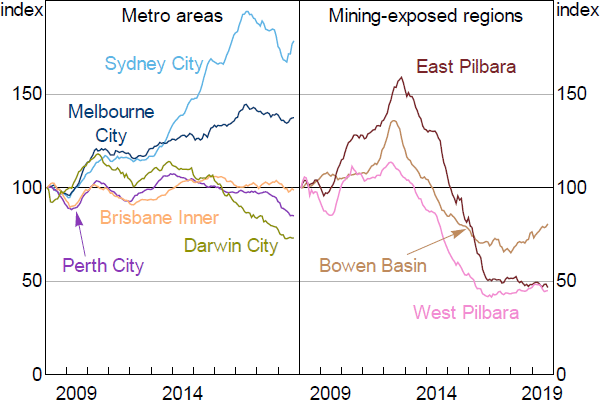
Hedonic regional housing price indices are sourced from CoreLogic. These data are available for Statistical Area Level 3 (SA3) regions (there are around 350 SA3 regions in Australia, each comprising between 20,000 and 130,000 residents). As at June 2019, housing prices had declined from their peaks in most regions (by around 8 per cent on average), but had fallen by as much as 70 per cent in some mining-exposed regions (Figure 1).
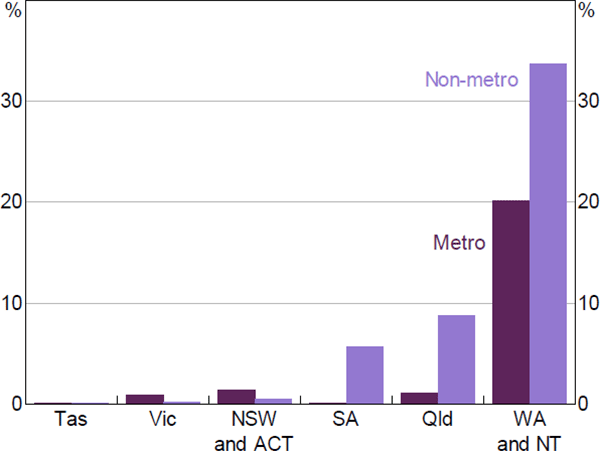
A loan is defined as having negative equity if its indexed LVR is above 100 (i.e. the estimated value of the property has fallen below the amount owing on the mortgage). The incidence of negative equity has been fairly rare in Australia, at around 4 per cent of the loans in the dataset in 2019.[4] These loans were mostly located in the mining-exposed regions of Western Australia, Queensland and the Northern Territory, and many were originated between 2012 and 2016 (Figure 2; see RBA (2019) for further details). Many of these loans were located in metropolitan Perth and Darwin. Note that I classify SA3 regions as mining-exposed if they contain at least two coal, copper or iron ore mines or if at least 3 per cent of the labour force is employed in the mining industry.
Sources: Author's calculations; CoreLogic data
Sources: ABS; Author's calculations; CoreLogic data; RBA; Securitisation System
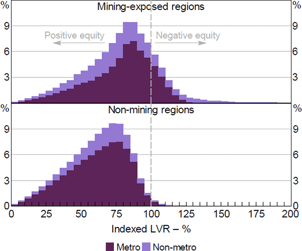
The extent of negative equity has also been greater in mining-exposed regions, particularly in non-metropolitan regions (Figure 3). Since the risk of foreclosure may increase nonlinearly with the extent of negative equity, regional mining areas play an important role in identifying the relationship between negative equity and default risk.
Sources: ABS; Author's calculations; CoreLogic data; RBA; Securitisation System
3.3 Census Data
Regional economic data are sourced from the ABS Census. Key among these is the regional unemployment rate. I use a version of the unemployment rate that adjusts for internal migration; it records the unemployment rate of working-age individuals in 2016, based on the SA3 region in which they lived at the previous census in 2011. Adjusting for internal migration is important in the context of the winding down of the mining investment boom, as many unemployed workers had migrated from mining regions to other areas in search of employment, particularly to capital cities. Unadjusted regional unemployment rates are a poor proxy for the true probability that home owners from mining-exposed areas experienced unemployment.[5]
4. Stylised Facts
The stylised facts in this section are consistent with the double-trigger hypothesis; arrears rates have a positive relationship with regional unemployment, and foreclosure rates are higher for loans with negative equity. But econometric modelling is still required to separately identify the two distinct triggers, not least because the regional incidence of unemployment and negative equity are correlated.
4.1 Entries to Arrears are Correlated with Regional Unemployment Rates
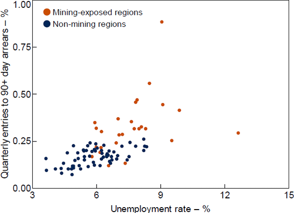
At the region level, entries to 90+ day arrears are positively correlated with unemployment rates; both tend to be higher in mining-exposed regions (Figure 4). The regions with the highest shares of loans entering arrears are ‘Outback Western Australia’ (particularly the Pilbara), ‘Outback Queensland’ and Mackay.
Notes: Entries to arrears are averaged over 2015–19; 2016 unemployment rate by usual place of residence in 2011; SA4 regions
Sources: ABS; Author's calculations; RBA; Securitisation System
4.2 Loans with Negative Equity are More Likely to Transition to Foreclosure
Transitions of loans from arrears, and the time they take to transition, are a function of both borrowers' and lenders' actions. In Australia, lenders issue borrowers with a notice of default once a loan enters 90+ day arrears (ASIC nd). Lenders may commence legal action to repossess the property if the borrower does not become fully current on their mortgage payments within the notice period, which is at least 30 days. The loan is defined as being in foreclosure once the ownership of the property has been transferred to the lender, and the lender will then make arrangements to sell the property. The lender may seek a court judgement for recourse to the borrower's other assets if the sale price of the property is insufficient to cover the amount owing plus foreclosure costs.
Under Australian consumer credit protection regulations, borrowers may submit a hardship application to their lender following the receipt of a notice of default, outlining why they are experiencing repayment difficulties, how long they expect their financial difficulties to continue and how much they can afford to repay. Lenders are required to consider hardship variations where cases are deemed to be genuine and meet certain requirements, and to provide alternatives such as repayment holidays or an extension of the loan term. Lenders will also typically delay legal proceedings when borrowers provide evidence that they are in the process of selling their property.
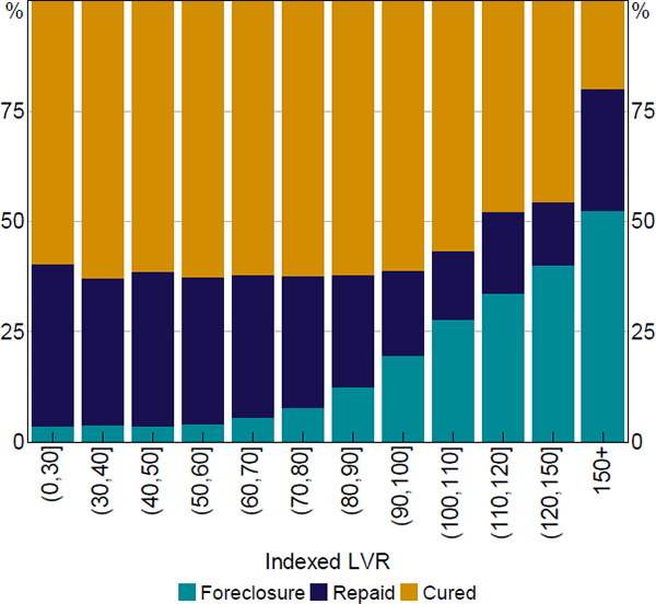
The transitions of loans from arrears are highly correlated with the loans' equity positions as at the time they entered arrears (Figure 5). Most loans with positive equity eventually cure (defined as becoming fully current on their scheduled payments) or are fully repaid (i.e. resolved through the borrower selling the property or refinancing). On the other hand, the share of loans that go on to foreclose is increasing in the degree of negative equity, as the borrower cannot profitably sell their property to avoid foreclosure and the probability that the value of negative equity exceeds the cost of foreclosure increases with the extent of negative equity. Loans in arrears that are deeply in negative equity have around a 50 per cent probability of eventually transitioning to foreclosure. Some readers may be surprised that this share is not higher; perceived foreclosure costs, full recourse to other assets (including other properties) and borrower expectations of a future housing price recovery may be contributing factors.[6]
Note: Final status of loans (excludes loans that remained in arrears at last observation)
Sources: Author's calculations; CoreLogic data; RBA; Securitisation System
Although foreclosure rates are higher for loans with high LVRs, by number the majority of foreclosed loans appear to have slightly positive equity when they enter arrears. Several factors may explain this, including that equity may have been mismeasured. Mismeasurement could occur if the loan balance does not capture all debts (such as subsequent accumulated balances in arrears or the presence of other debts) or because the property valuation is only an estimate. Nonetheless, it appears that some loans proceed to foreclosure with positive equity.
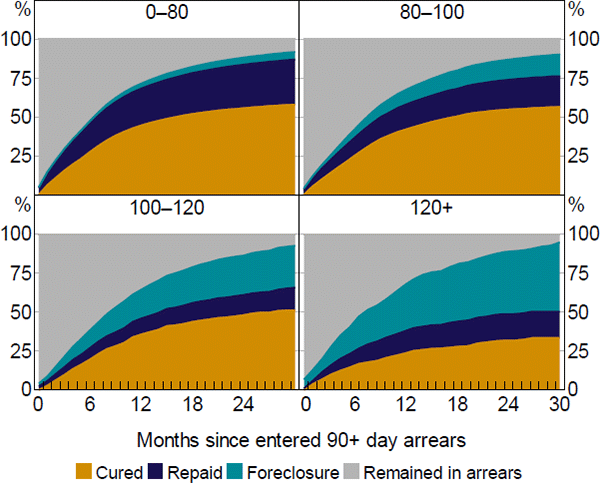
Transitioning from arrears can be a slow process. Among loans that transition from arrears within the sample period, the median loan that fully repays (refinances or sells the property) takes three months to do so, while the median loan that either cures or enters foreclosure takes six months to do so (Figure 6). Some loans take significantly longer to transition from arrears. Restructuring arrangements arising from hardship applications may assist loans with curing (fewer loans with restructuring arrangements proceed to foreclosure), but may also prolong the time a loan spends in arrears. More generally, lenders may exercise some degree of leniency when they expect to receive better rates of return through the borrower resolving their situation than through a forced sale.
Note: First arrears events
Sources: Author's calculations; CoreLogic data; RBA; Securitisation System
While foreclosures in the absence of 90+ day arrears are relatively rare, in line with banks' standard foreclosure procedures and the double-trigger hypothesis, they do occur. Around 4 per cent of foreclosures occur without a 90+ day arrears spell being observed during the sample period; most of these loans appear to have a prolonged history of multiple arrears spells of less than 90 days.[7]
5. Estimation Strategy
5.1 A Two-stage Approach
The simplest version of the double-trigger hypothesis states that both an ability-to-pay shock and negative equity are required for a loan to default, and can be represented in Equation (2):
where Fi,t is the binary foreclosure event at time t for loan i, Ai,t is the extent of the ability-to-pay shock, Ni,t is the extent of negative equity, and and are some thresholds.
Equation (2) states that a borrower forecloses on their mortgage only if:
- the borrower experiences a ‘shock’ to their ability to repay their mortgage that exceeds some threshold of their ability or willingness to pay, and
- negative equity on the mortgage exceeds some threshold of negative equity that the borrower is willing to tolerate, given their individual costs of foreclosure.
If either the ability-to-pay shock or the extent of negative equity do not exceed these thresholds, the double-trigger hypothesis predicts that the borrower will not foreclose.
Note that the borrower would be willing to enter foreclosure as soon as the conditions of Equation (2a) are met. However, the timing of foreclosure is also determined by the lender, which faces incomplete information regarding the situation and preferences of the borrower. Where a lender extends some leniency towards the borrower, foreclosure will not occur immediately upon Equation (2a) being satisfied. Where this is the case, the borrower may not proceed to foreclosure at all if the ability-to-pay shock or negative equity are subsequently reversed. Hence, the probability of foreclosure in Equation (2a) is greater than 0, rather than equal to 1.
The probability of foreclosure can be further decomposed into the probability that a loan forecloses given that it has been in 90+ day arrears, R90+i,t−1 = 1, plus the probability that it proceeds straight to foreclosure:
As noted above, in Australia most loans proceed to foreclosure only after a notice of default has been served, which occurs after the loan enters 90+ day arrears. Therefore, and Equation (3) collapses to:
It is sufficient to estimate Equation (4) to examine the determinants of foreclosures. Notice that Equation (4) can be estimated separately in two stages: the probability that a loan enters 90+ day arrears and the probability that a loan forecloses, conditional on having been in 90+ day arrears.
This two-stage framework is well suited to testing the double-trigger hypothesis, which is naturally described in two stages:
- A ‘shock’ to the borrower's ability to repay the mortgage causes the borrower to miss repayments and enter arrears.
-
The loan's transition from arrears depends on:
- the ability-to-pay shock – if the ability-to-pay shock is subsequently reversed, the borrower may become current on payments and cure
-
the loan's equity position:
- if the loan has positive equity, the borrower can profitably sell their property to avoid foreclosure
- if the loan has negative equity, but to a lesser extent than the cost of foreclosure, the borrower may minimise losses by selling the property themselves to avoid foreclosure
- if the loan has negative equity in excess of the cost of foreclosure, the loan may go on to foreclosure.
A two-stage modelling approach allows the full set of predictions from the double-trigger hypothesis to be tested – including an analysis of the loans that cure and repay, rather than just those that foreclose. This acknowledges that the transition from arrears to foreclosure is not automatic; rather most loans in arrears do not go on to foreclosure and the actions of both borrowers and lenders influence this transition.
Testable sub-hypotheses that arise from the above are:
Hypotheses A and B relate to the first stage. Hypothesis A states that the probability of a loan entering 90+ day arrears is increasing in the size of the ability-to-pay shock and is close to 0 where the size of the shock does not exceed the borrowers' ability-to-pay threshold. Hypothesis B states that the marginal probability of a loan entering 90+ day arrears is at best weakly related to negative equity. Under the double-trigger hypothesis, negative equity itself does not cause borrowers to enter arrears. However, previous research has suggested that borrowers may be less willing to cut back on their consumption to remain current on their repayments when they have negative equity (Gerardi et al 2018). If this is the case, then threshold may be a function of Ni,t and the derivative in Hypothesis B may be positive.
Hypotheses C and D relate to the second stage. Hypothesis C states that the probability of foreclosure is increasing in the extent of negative equity, given that the loan has been in arrears, but is close to 0 where the extent of negative equity is less than the cost of foreclosure. Hypothesis D states that once a loan has arrears of 90+ days, the size of the ability-to-pay shock has no influence on the probability of foreclosure (unless the shock is subsequently reversed).
5.2 Cox Proportional Hazard Models
I test the hypotheses outlined above using a two-stage Cox proportional hazard model framework with competing risks. Following the framework set out above, the first stage examines entries to 90+ day arrears, while the second stage estimates transitions to foreclosure, curing and full repayment.
Cox proportional hazard models are most commonly used in the biomedical literature, but have also been used to estimate the effect of covariates on the probability of loans entering arrears (e.g. Deng et al 1996; Gerardi et al 2008). They estimate the effect of a change in a vector of variables on the instantaneous probability (or hazard) that an event of interest is observed, given that event has not yet been observed (Cox 1972).
The Cox proportional hazard model is useful when the probability of an event changes over some time dimension (such as time since loan origination), loans are observed at different points along this time dimension, and those loans that have not yet experienced the event could still do so in the future (known as right censoring). The key virtue of the Cox model is that this time dimension is part of the inherent structure of the model, as opposed to binary or multinomial choice models that include the time dimension as an additional component with a specific functional form. With this time-based structure, the Cox model is not biased by not having information about the future; all that is necessary is knowledge of whether the event had occurred by the point at which the loan was observed.
One downside of the Cox model is that outcomes that prevent the event of interest from occurring (known as competing risks) are treated as if the loans were right censored. For example, a loan that is repaid early is treated as if it could still go into arrears in the future. This is problematic if the factors that cause loans to be repaid are related to the factors that cause arrears (i.e. the events are not independent). While models exist that incorporate the time dimension in a similarly flexible way to the Cox model but do not treat competing risks as independent, these models can be difficult to interpret and are not commonly used in the empirical mortgage default literature.[8] So I use the Cox model.[9]
The Cox model takes the form specified in Equation (5), where is the baseline hazard (instantaneous probability) of event E occurring at time t, x is a vector of explanatory variables and is a vector of coefficients. The model flexibly accounts for the effect of time on the hazard of experiencing the event of interest by only specifying results relative to a baseline probability (the baseline hazard rate). By assuming the covariates affect the hazard rate multiplicatively, the baseline hazard rate need not be specified in order to estimate how the covariates change the probability of the event of interest.
The results reported in Section 6 are the ‘hazard ratios’ from the estimated models (these ratios are used to test the hypotheses derived in Section 5.1). Hazard ratios, similar to odds ratios, can be interpreted as a one unit increase in variable k leading to a per cent increase in the probability of event E above the baseline hazard at time t. For example, a hazard ratio of 1.7 would represent a 70 per cent increase in the instantaneous probability of an outcome. The virtue of reporting results in this way is that hazard ratios do not depend on t or the value of xit. Note that the exp function imposes a multiplicative relationship between the x variables.
5.3 Model Specification – Further Details
5.3.1 Model details – dependent variables, competing risks and sample construction
In the first-stage model, the event of interest is a loan entering 90+ day arrears, the competing risk is a loan being fully repaid, and the time dimension is seasoning (i.e. the time since origination). Loans which were ‘performing’ (i.e. not in arrears), were less than 90 days in arrears as at June 2019, or that were removed from the dataset for some other reason, are also treated as right censored.[10] To avoid problems with left censored data (i.e. loans experiencing an event prior to entering the dataset), I exclude loans originated prior to 2013.[11] This results in a sample of 1.7 million loans. To allow for the inclusion of time-varying covariates that may be correlated with seasoning, such as indexed LVRs and changes to required loan repayments, the model is estimated using quarterly observations.[12]
The second stage is estimated on loans that have entered 90+ day arrears. In the second stage, there are three possible events (foreclosure, curing or full repayment). For most of my results, and when testing the hypotheses, foreclosure is the event of interest.[13] The time dimension in this stage is the time since entering 90+ day arrears. Loans which remained in arrears as at June 2019, had a competing event occur, or that were removed from the sample for other reasons while still in arrears, are treated as right censored. I exclude loans that were in arrears at the beginning of the sample, as the length of their time in arrears is unknown. Time-varying explanatory variables, such as LVRs, are included as at the time the loan entered arrears (so they are not correlated with the time dimension in the second stage).
The two stages are estimated independently. As shown in Equation (4), independent estimation is sufficient to examine the double-trigger hypothesis and the determinants of foreclosure; incorporating the first stage results into the second stage using a Heckman selection procedure is not necessary. That said, this set-up means that the second stage results alone cannot be used to make statements about the unconditional probability of foreclosure.
Relatedly, all of my results are relative to a baseline hazard. This means that a hazard ratio of 1.7 for a particular variable, for example, only tells you that the hazard is 70 per cent higher with the increase in that variable; it provides no information about the probability of the event occurring. Where the baseline hazard is close to 0, large hazard ratios are required for the overall probability to move meaningfully away from 0.
5.3.2 Key explanatory variables
The key ability-to-pay explanatory variable is the regional unemployment rate, adjusted for internal migration. This is used as a proxy for the probability that an individual borrower faces an ability-to-pay shock.[14] As with many other empirical studies, actual individual shocks cannot be observed in the data. This means that the true effect of becoming unemployed (or facing another individual shock) will be underestimated by the models, possibly by a very large degree. Notwithstanding this, the estimated hazard ratio for the unemployment rate is expected to be particularly large in the first-stage model, as unemployment represents a large ability-to-pay shock. While the unemployment rate is expected to be of secondary importance in the second stage, as it is not expected to affect foreclosure (conditional on being in arrears), it may still be relevant as regaining employment may allow a borrower to cure (a competing risk).
Two variables may be related to a borrower's ability-to-pay threshold. The first of these is the debt serviceability ratio (DSR); in the event of a reduction in income, a borrower with low relative servicing costs may be able to continue to make repayments from their remaining income or to draw on savings for a longer period to make repayments.[15] The second is mortgage repayment buffers; a borrower with sizeable accumulated excess repayments may be able to draw down on these repayments for a number of months before the loan enters arrears.[16] As such, a low serviceability ratio and high repayment buffers may enhance a borrower's resilience to shocks.
Equity is measured by indexed scheduled LVR, which is specified as buckets in the model. Each bucket is treated as a separate variable; for example, a loan with an LVR of 76 would have a value of one in the 70–80 LVR bucket and a value of zero in all other LVR buckets. The use of buckets is standard within the literature as it is flexible and can highlight any potential nonlinearities or threshold effects. The double-trigger hypothesis predicts that foreclosure occurs for loans in arrears when . But individual borrowers' foreclosure cost thresholds are not observable; this implies that the estimated hazard ratio for negative equity may be increasing nonlinearly, as it becomes increasingly likely that a higher Ni,t exceeds for more borrowers.
One potential criticism of models that include a number of regional variables is that the variables may be correlated, making the identification of individual effects difficult. Of particular concern may be the potential correlation between regional unemployment rates and housing prices, which are incorporated in the indexed LVR estimates. Very large sample sizes (approximately 12 million observations in the first stage and 40 thousand in the second stage), and the estimation of indexed LVRs at the individual loan level, help alleviate this concern. In addition, state and time fixed effects have been added to the models and standard errors are clustered at the SA3 region level.
Various loan-level controls are also included, such as borrower and loan characteristics. Variable definitions can be found in Appendix A.
6. Results
Table 1 shows the key results from the first- and second-stage models. Full results are available in Appendix B and results are discussed in detail below.[17] Overall, estimated hazard ratios tend to be larger for ability-to-pay factors in the first stage while hazard ratios for equity are larger in the second stage. Concordance ratios of 0.79 in both stages indicate that the total explanatory power could be considered moderate, and most of the explanatory power is contributed by the main variables of interest.[18] However, unobserved characteristics and events may also be important – shocks may be idiosyncratic (such as illness), the unemployment rate is only a weak proxy for individual unemployment and borrower foreclosure costs are likely to be heterogeneous.
| Explanatory variable | Stage 1: entries to 90+ day arrears | Stage 2: transitions to foreclosure |
|---|---|---|
| Ability-to-pay factors | ||
| Change in ability to pay | ||
| Unemployment rate(a) | 1.21*** | 1.13* |
| Socio-economic index | 1.00*** | 1.00 |
| Mining share of employment | 1.02*** | 1.00 |
| Interest-only (IO) period expired | 1.94*** | 1.03 |
| Change in interest rates (selected; base = 0) | ||
| +2 to 25 bps | 1.03 | na |
| Over +25 bps | 1.19*** | na |
| Multiple debtors | 0.73*** | 0.77*** |
| Ability-to-pay threshold | ||
| Repayment buffer (base = 1–6 months) | ||
| Under 1 month | 2.32*** | na |
| Over 6 months | 0.33*** | na |
| DSR (base = 10–20) | ||
| 0–10 | 0.61*** | 1.17 |
| 20–30 | 1.42*** | 0.83* |
| 30–40 | 1.80*** | 0.82 |
| 40+ | 1.93*** | 0.89 |
| Equity and housing market factors | ||
| Indexed LVR buckets (selected; base = 60–70) | ||
| 30–40 | 0.78*** | 0.76 |
| 70–80 | 1.14*** | 1.17 |
| 80–90 | 1.32*** | 1.69*** |
| 90–100 | 1.49*** | 2.10*** |
| 100–110 | 1.87*** | 2.52*** |
| 110–120 | 2.01*** | 3.26*** |
| 120–150 | 2.13*** | 3.44*** |
| 150–200 | 2.73*** | 4.60*** |
| 200+ | 3.30*** | 7.54*** |
| Turnover ratio | 1.01 | 0.92*** |
| Remote region | 1.34*** | 1.56*** |
| Loan/borrower characteristics | ||
| Self-employed | 1.19*** | 1.06 |
| Investor | 0.67*** | 1.33*** |
| IO | 0.79*** | 1.20** |
| Low documentation | 2.01*** | 1.08 |
| No of observations | 12,370,400 | 42,100 |
| No of events | 19,600 | 2,400 |
| Concordance ratio | 0.79 | 0.79 |
|
Notes: ***, ** and * denote statistical significance at the 0.1, 1 and 5 per cent levels, respectively (a) From model excluding the socio-economic index Sources: ABS; Author's calculations; CoreLogic data; RBA; Securitisation System |
||
6.1 First-stage Hazard Model: Entries to 90+ Day Arrears
6.1.1 Ability-to-pay factors
The model results suggest that both ability-to-pay shocks and ability-to-pay thresholds play a key role in determining entries of loans into 90+ day arrears. These results are consistent with Hypothesis A.
6.1.1.1 Ability-to-pay shocks
Three variables in the model proxy for the probability that a borrower experiences an ability-to-pay shock: the regional unemployment rate, the regional share of mining employment and the regional socio-economic index. Since these variables each incorporate labour market dynamics, they are correlated with each other. At the extreme, the regional socio-economic index is a composite index of indicators, and a large component is the regional unemployment rate (the correlation coefficient is –0.65). So their effects should be evaluated together; the simplest way to do this is to re-estimate the model to exclude the correlated variable.[19]
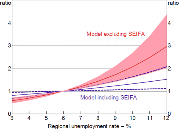
The hazard ratios estimated for the regional unemployment rate are large in magnitude and statistically significant. This is particularly the case when the socio-economic index is excluded from the model, with estimates suggesting that every 1 percentage point increase in the regional unemployment rate increases the hazard of a loan entering 90+ day arrears by 21 per cent.[20] Taking into account the wide distribution of unemployment rates across regions, this implies that loans in regions with high unemployment rates are up to four times more likely to enter arrears than loans in regions with low unemployment rates (Figure 7). Simulations by Gyourko and Tracy (2014) show that using regional unemployment rates as a proxy for individual unemployment spells may underestimate the true effect of becoming unemployed by a factor of 100 – suggesting that the role of unemployment in entries to arrears may be very large.
Notes: Hazard ratio set to 1 at the median value of x variable; shaded area/dashed lines denote 95% confidence intervals
Sources: ABS; Author's calculations; CoreLogic data; RBA; Securitisation System
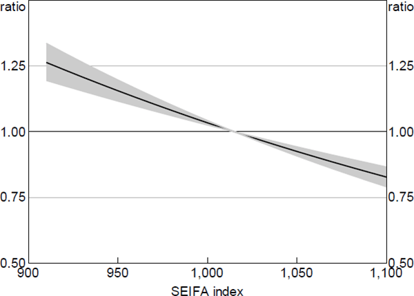
The socio-economic profile of a region may be correlated with borrowers' probability of experiencing an ability-to-pay shock, and the severity of the shock, to the extent that it is correlated with unobserved borrower characteristics such as age, security of employment, financial literacy and understanding of the legal system. For example, Mincer (1991) finds that younger and less educated workers tend to suffer larger and more persistent employment loss during recessions – the effect of which may not be fully captured in the regional unemployment rate. Lower financial literacy may also be correlated with the presence of consumer debts, such as credit cards, that may lower borrowers' ability-to-pay threshold (Disney and Gathergood 2013). Holding all other covariates (including the regional unemployment rate) constant, loans located in postcodes with the highest socio-economic indices (SEIFA) were around 40 per cent less likely to enter arrears than those located in regions with low SEIFA (Figure 8).[21]
The share of regional employment in the mining industry is also strongly correlated with entries to arrears, even after controlling for regional unemployment rates. This may be related to reductions in income or lower job security beyond that indicated by regional unemployment rates, although we cannot rule out the possibility that mining regions may differ systematically in some other respect (see Section 7.2 for a discussion). Loans located in regions with the highest mining shares of employment were estimated to be twice as likely to enter arrears as those in regions with fewer jobs in the mining industry (Figure 9).
Notes: Hazard ratio set to 1 at the median value of x variable; shaded area denotes 95% confidence intervals
Sources: ABS; Author's calculations; CoreLogic data; RBA; Securitisation System
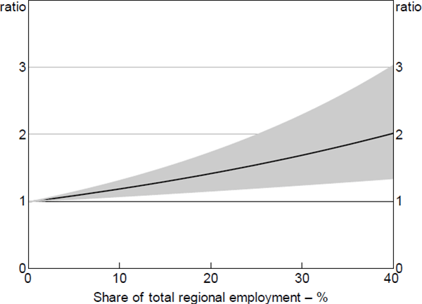
Notes: Hazard ratio set to 1 at the median value of x variable; shaded area denotes 95% confidence intervals
Sources: ABS; Author's calculations; CoreLogic data; RBA; Securitisation System
Borrower characteristics that are likely to be correlated with variability in income – and the probability of facing an ability-to-pay shock – were also positively correlated with the probability of entering arrears. Self-employed borrowers were estimated to be 19 per cent more likely to enter 90+ day arrears, consistent with these borrowers sometimes having less stable sources of income compared to employees. By contrast, mortgages backed by multiple borrowers were 27 per cent less likely to enter arrears; it is unlikely that all borrowers simultaneously experience an income reduction.
Increases in required loan repayments may cause liquidity-constrained borrowers to enter arrears, even without notable changes to their earnings. The magnitude of their effect on a borrower's ability to pay, however, would generally be less than that of the typical unemployment spell. Increases in required loan repayments are the only reduction to borrowers' ability to pay that we can directly observe in the data.
There have been two notable sources of increases to required repayments for borrowers over the sample period. First, lenders raised their standard variable rates for investor and interest-only (IO) loans in 2015 and 2017, typically by between 20 and 100 basis points (Kent 2017; Kohler 2017).[22] Second, a growing share of IO loans have had their IO periods expire over recent years, resulting in a step-up in total required payments by around 30 to 40 per cent for those loans (Kent 2018). To capture these effects, two variables have been included in the model: lagged changes in interest rates, expressed in buckets, and an IO period expiry indicator variable.
The model estimates suggest that an increase in interest rates in excess of 25 basis points was associated with a 19 per cent increase in the hazard of loans entering 90+ day arrears, relative to loans whose interest rate was unchanged. Most borrowers facing IO period expiries were able to transition to higher repayments without encountering repayment difficulties. Notwithstanding this, estimates suggest that borrowers whose IO period had expired in the previous six months were twice as likely to enter arrears compared to other loans paying principal and interest. However, this coefficient is likely to be upwardly biased due to selection bias – loans facing an IO period expiry may be riskier on dimensions other than those captured in the model.[23]
6.1.1.2 Ability-to-pay thresholds
Under the double-trigger hypothesis, various factors may influence the ability-to-pay threshold, that is, the size of the ability-to-pay shock that a borrower is able to tolerate before entering arrears. These include buffers that borrowers have built up through their loan repayments and savings, as well as the ratio of their loan repayments to income.
Borrowers who are ahead of their loan repayments may draw down upon their prepayment buffers in the event of an ability-to-pay shock, extending the time until they are behind on their repayment schedules. This may allow a borrower to avoid arrears, effectively raising the ability-to-pay threshold. The median borrower in the sample had a maximum of between one and six months of buffers at some point in time. Relative to the median borrower, borrowers who have ever had a buffer of over six months were 67 per cent less likely to enter 90+ day arrears, while a borrower who has never had a buffer greater than one month was 2.3 times more likely to enter arrears.
Likewise, loan serviceability affects the ability-to-pay threshold – borrowers facing a mild income shock may be able to continue making repayments if they have a low DSR, but are increasingly unlikely to be able to do so for higher DSRs. Model estimates suggest that this effect is important, with loans with high DSRs being around three times as likely to enter arrears as loans with low DSRs (Figure 10).[24],[25]
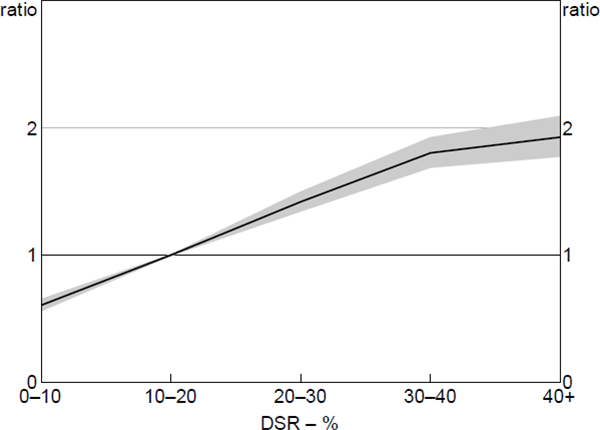
Notes: Hazard ratio set to 1 at the median value of x variable; shaded area denotes 95% confidence intervals
Sources: ABS; Author's calculations; CoreLogic data; RBA; Securitisation System
6.1.2 Equity
As highlighted in Hypothesis B, the double-trigger hypothesis implies no direct link between equity and entries to arrears. However, the probability of entering arrears may be weakly increasing in negative equity if borrowers' willingness to repay threshold is a function of equity. Empirical research by Gerardi et al (2018) suggests that borrowers facing an ability-to-pay shock may attempt to avoid arrears, and ultimately foreclosure, by cutting back on consumption expenditure if they have positive equity.[26]
The model estimates of the magnitude of the relationship between negative equity and entries to 90+ day arrears are surprisingly large; a loan that is deeply in negative equity was three times as likely to enter arrears as a loan with the median indexed LVR (Figure 11). The buckets specification is flexible enough to highlight nonlinearities. The probability of entering arrears increases gradually for loans with LVRs above 50, but does not accelerate for loans with negative equity. It is possible that this result may reflect a correlation with ability-to-pay factors that have not been fully controlled for, such as changes in borrower income. This means that the equity result is inconclusive; it is not sufficient to refute the double-trigger hypothesis, but it also does not rule out the possibility that some borrowers with negative equity may strategically default.
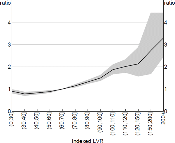
Notes: Hazard ratio set to 1 at the median value of x variable; shaded area denotes 95% confidence intervals
Sources: ABS; Author's calculations; CoreLogic data; RBA; Securitisation System
The above ability-to-pay results confirm Hypothesis A, whereas the surprisingly large hazard ratios for equity prevent me from confirming Hypothesis B. That said, there may be unobserved ability-to-pay factors that are correlated with equity, and the ability-to-pay hazard ratios are larger than the equity hazard ratios. Therefore, the first stage results are broadly consistent with the double-trigger hypothesis.
6.2 Second-stage Hazard Model: Transitions from Arrears
6.2.1 Equity and housing market turnover
The double-trigger hypothesis predicts that the degree of negative equity is the main determinant of whether a loan in arrears transitions to foreclosure. Consistent with Hypothesis C, model estimates suggest that the probability of loans transitioning into foreclosure is increasing in the degree of negative equity. Meanwhile, the probability of loans curing or fully repaying declines for loans with negative equity. Loans that are deeply in negative equity (at the point of entering arrears) are around five to eight times as likely to transition to foreclosure as a loan with the median LVR (Figure 12). The magnitudes of these hazard ratios are larger than in the first stage results. There are no distinct thresholds around which loans transition to foreclosure, in line with international evidence that suggests that borrowers have heterogeneous foreclosure costs and housing price expectations (Guiso et al 2013; Bhutta et al 2017).
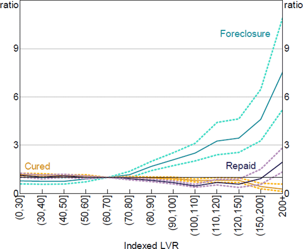
Notes: Hazard ratio set to 1 at the median value of x variable; dashed lines denote 95% confidence intervals
Sources: ABS; Author's calculations; CoreLogic data; RBA; Securitisation System
Although low turnover in a region may be symptomatic of other problems in that region, low turnover itself may also affect whether a borrower is able to avoid foreclosure by selling the property themselves. There are several channels through which this may occur, including by hampering price discovery, slowing sale times, increasing housing price variance (thereby increasing the probability that a loan has negative equity), and sending a negative signal to potential buyers (e.g. about the quality of properties on the market). Even after controlling for region remoteness and indexed LVRs, loans located in areas with lower turnover ratios (which were often regional areas) were around 40 per cent more likely to transition to foreclosure than those in areas with high turnover ratios (Figure 13). They were also less likely to be fully repaid. These results suggest that nonlinearities may be a risk in a housing market stress scenario, where low housing turnover may exacerbate foreclosures.
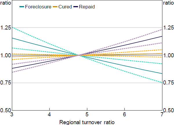
Notes: Hazard ratio set to 1 at the median value of x variable; dashed lines denote 95% confidence intervals
Sources: ABS; Author's calculations; CoreLogic data; RBA; Securitisation System
In addition to these effects, loans in regional towns and remote areas were around 50 per cent more likely to proceed to foreclosure than their counterparts in larger cities (all else equal), and were less likely to fully repay. This might be due to nonlinearities in housing market conditions, such as borrowers having lower housing price growth expectations or through longer sale times not being fully accounted for by the housing turnover ratio. Alternatively, it may reflect slower recovery times from ability-to-pay shocks in regional areas due to shallower labour markets.
6.2.2 Ability-to-pay factors
The hazard ratios for ability-to-pay factors in the second-stage model for foreclosures were not statistically significant and were small in magnitude, with the exception of the regional unemployment rate (Figure 14). These results are consistent with the double-trigger hypothesis and in line with Hypothesis D, that is, the size of the ability-to-pay shock is not relevant for transitions to foreclosures, but a reversal of the shock (e.g. the borrower regaining employment) may allow the borrower to cure.
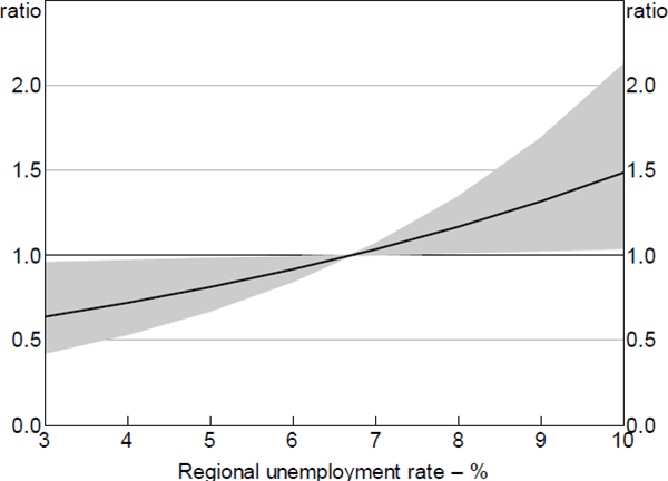
Notes: Model excluding the SEIFA variable; hazard ratio set to 1 at the median value of x variable; shaded area denotes 95% confidence intervals
Sources: ABS; Author's calculations; CoreLogic data; RBA; Securitisation System
International evidence suggests that a higher unemployment rate impairs a borrower's ability to cure by regaining employment. For example, Adelino et al (2013) point to the rise in the unemployment rate as a factor in the reduction in cure rates in the United States from around 70 per cent to 25 per cent between 2006 and 2009. However, the hazard ratio estimated in my model for loan cures was relatively small in magnitude; the regional unemployment rate being a poor proxy for individual unemployment may again make it difficult to estimate the true effect of unemployment.
6.2.3 Recourse
It is likely that full recourse to borrowers' other assets is a significant deterrent to foreclosure in Australia, however, its effect is difficult to measure in the absence of data on borrowers' other assets and debts. In jurisdictions with full recourse, borrowers' total equity position should be measured by their total debt-to-assets ratio, rather than indexed LVR. While this information is not available in the Securitisation Dataset (or in most loan-level datasets used in international studies), several variables may be partial proxies.
Investors and borrowers with high incomes may be likely candidates to have other assets that may have positive net worth and therefore reduce the borrowers' probability of foreclosure for a given indexed LVR. The results do not support this hypothesis. The hazard ratio for the high income dummy is not statistically significant in the second-stage model. Further, while investors were less likely to enter arrears in the first-stage model, having entered arrears, they were more likely to proceed to foreclosure in the second-stage model.[27] A number of competing factors may explain this result. For example, Albanesi, De Giorgi and Nosal (2017) argue that investors may be more likely to take on more risks or be more strategic in their decision-making due to a lack of sentimental attachment to the property or moving costs.
6.2.4 Restructuring arrangements
An important control in the second-stage model is whether the borrower had obtained any restructuring arrangements (including through hardship provisions), which are designed to assist the borrower with curing. Restructuring arrangements reduced the hazard of foreclosure by 60 per cent for the full subset of loans, and by 40 per cent for loans with negative equity. As well as increasing the likelihood of a loan in 90+ day arrears curing, restructuring arrangements also extend the time that loans spend in arrears.
7. Discussion
7.1 Assessing the Contributions of Ability-to-pay Factors and Negative Equity
To understand the contributions of ability-to-pay factors and negative equity to mortgage defaults, we need to go beyond evaluating the sign of the hazard ratios. The contributions of each variable will depend on both the magnitude of the hazard ratios and the distributions of the observed data. For example, a hazard ratio for a particular characteristic may be very large, but if that characteristic does not exhibit much variation, including among the set of loans that default, then it cannot be considered an economically significant driver of mortgage defaults. However, determining the share of total variation explained by each variable is difficult in multiplicative models such as Cox models.
This section evaluates the contributions by considering the change in the estimated hazard ratio for each variable generated by moving across the distribution of the variable (from one percentile to another). The interquartile range provides a useful guide to the role of variables over their typical ranges, while the difference between the 1st and 99th percentile gauges the influence of particularly risky loan characteristics and stressed economic conditions. These results are shown in Figures 15 and 16, where bars represent the relative hazard ratios for the interquartile ranges and dots are the difference between the 1st and 99th percentiles.[28] To assist visual inspection, relative hazard ratios that are less than 1 are inverted to standardise the scales, which can be interpreted as the change in risk involved in moving from the less risky characteristic to the more risky characteristic.
First-stage relative hazard ratios for the interquartile ranges of the data were largest for ability-to-pay factors (Figure 15). The largest relative hazard ratio was for repayment buffers, where mortgages with buffers of less than one month were 7 times more likely to enter arrears than those with buffers greater than six months, and both outcomes were common. Relative hazard ratios for other key ability-to-pay factors (unemployment rate, DSR, multiple debtors) were more moderate at around 1.4 – that is, moving from the 25th to the 75th percentile of the variable led to around a 40 per cent increase in the hazard of entering arrears. While these estimates are individually moderate in magnitude, the model is multiplicative and a combination of risk factors may still generate a large change in the hazard of entering arrears. The relative hazard ratio for indexed LVRs was slightly smaller, at 1.3.
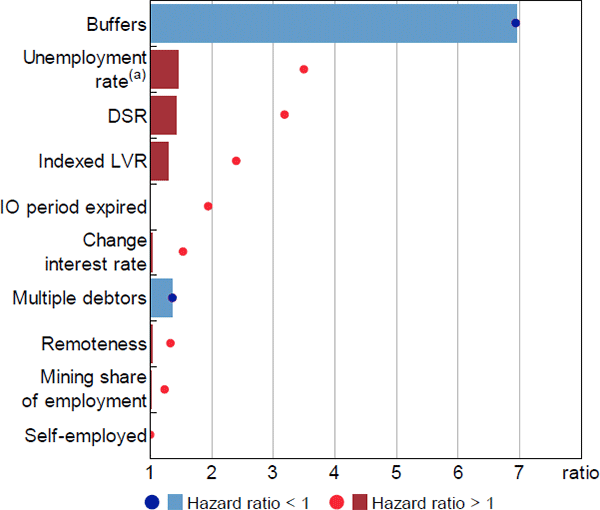
Notes:
Dots represent the relative hazard ratio of the 99th percentile observation to the 1st percentile; bars represent the interquartile range; hazard ratios that are less than 1 are inverted
(a) Estimate from model excluding the SEIFA variable
Sources: ABS; Author's calculations; CoreLogic data; RBA; Securitisation System
Whether ranking effects by the interquartile range or the tails of the distribution, ability-to-pay factors had the largest effects in the first-stage model. This is particularly noteworthy, since many of these variables are only proxies for an ability-to-pay shock or threshold and their effects are likely underestimated. This suggests that ability-to-pay factors can be considered the most important determinants of entries to 90+ day arrears, whether one is concerned about regular economic conditions or stressed economic conditions. Relative hazard ratios for equity were somewhat smaller, including in the comparison of the 1st and 99th percentiles, and therefore may not be considered the main determinants of entries to arrears – consider that only 7 per cent of loans that entered arrears had negative equity of any degree (Table A1).
In contrast, equity (indexed LVR) had the largest relative hazard ratio in the second-stage model for foreclosures, whether judged by the interquartile range or the tails of the distribution (Figure 16). This reflects both the larger estimated hazard ratios for indexed LVRs in the second-stage model, as well as the greater prevalence of negative equity among loans in arrears. At the tails of the distribution, the unemployment rate and turnover ratio had the next largest relative hazard ratios, while relative hazard ratios were small for most other variables in this model.
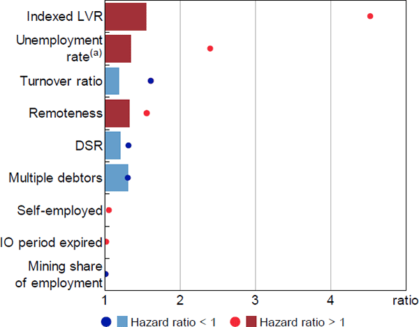
Notes:
Dots represent the relative hazard ratio of the 99th percentile observation to the 1st percentile; bars represent the interquartile range; hazard ratios that are less than 1 are inverted
(a) Estimate from model excluding the SEIFA variable
Sources: ABS; Author's calculations; CoreLogic data; RBA; Securitisation System
Overall, these results are also consistent with the double-trigger hypothesis – ability-to-pay factors appear to be the most important determinants of entries to arrears and negative equity of transitions to foreclosure.
7.2 The Applicability of Regional Shocks
In my analysis, insights regarding the macroeconomic determinants of mortgage defaults largely come from mining-exposed regions, which have experienced both increases in unemployment rates and declines in housing prices. Most of the loans in negative equity, particularly those with substantial degrees of negative equity, are located in mining regions. Any conclusions regarding mortgage defaults in stressed conditions, or the role of negative equity, therefore load heavily on mortgages in mining-exposed regions and the nature of the regional economic shock.
While insights from regional shocks are likely to be applicable to a more widespread shock in many ways, they may vary along several dimensions. Some of these possible dimensions are noted below. Overall, it is difficult to determine ex ante whether a regional shock may have more or less severe consequences for mortgage defaults than a broader shock.
- The response of macroeconomic policy to a broader shock may be stronger than for a regional shock, reducing the overall severity of a broader shock. While this may change the range of macroeconomic outcomes experienced, it is not clear that this would change the estimated model coefficients, unless there are nonlinearities or omitted variables.
- Internal migration may mitigate the severity of a regional shock if displaced workers can move to other regions to find work (albeit possibly at lower wages), but they may not have this option in a severe widespread shock. As a result, unemployment spells may be shorter in regional shocks, increasing the chance that borrowers are able to avoid arrears or subsequently cure. If this is the case, then the estimated coefficients on the labour market variables may underestimate their effect in a broader stress scenario, although this is mitigated by adjusting for internal migration in the unemployment rate measure.
- Regional housing market shocks may be more severe than national shocks and borrowers in remote regions may be less optimistic about a price recovery. Housing prices have fallen by around 70 per cent from their peak in some mining-exposed regions, more than double the nationwide US housing price decline during the financial crisis (although this could be due to the macroeconomic policy response in the United States). In addition, housing turnover rates are typically lower in non-metropolitan regions, which may exacerbate the severity of regional housing market shocks. Hence the probability of foreclosure may be higher at all LVR levels in a regional shock.
- Falls in asset prices may be broader in a widespread stress event than in a regional downturn, with declines across asset types and across housing market regions. This raises the probability that a borrower with negative equity on one asset has negative equity overall, and may mean that the risk of foreclosure for loans with negative equity has been underestimated.[29]
- Borrowers in metropolitan and non-metropolitan regions may vary along characteristics other than those captured in the models. For example, they may have different risk tolerances or variability in income that are not captured in regional aggregates.
To test for the representativeness of the mining region results, we can compare results from models estimated separately for mining and non-mining regions. This provides some surety about the results over the common ranges of the data, but does not guarantee results outside of these bounds (and this is still only a comparison of regional, rather than widespread, shocks).
In the first-stage model, estimated hazard ratios were similar for the key variables of interest. To the extent that there were differences, non-mining estimates tended to be slightly larger, although these differences were not statistically significant (Figure 17). In contrast, estimates of the baseline hazard suggest that the probability of the median loan entering arrears is slightly higher in mining regions (Figure 18).[30] This may indicate that unobservable characteristics, whether related to the borrowers or the macroeconomic environment, have increased the riskiness of loans located in mining regions. Notwithstanding this, the similarity of the hazard ratio estimates between the two models across the common data ranges suggests that the regional shock also likely provides plausible estimates and useful identification outside of these ranges.
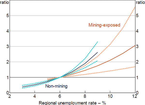
Notes: Model excluding the SEIFA variable; hazard ratio set to 1 at the median value of x variable; dashed lines denote 95% confidence intervals
Sources: ABS; Author's calculations; CoreLogic data; RBA; Securitisation System
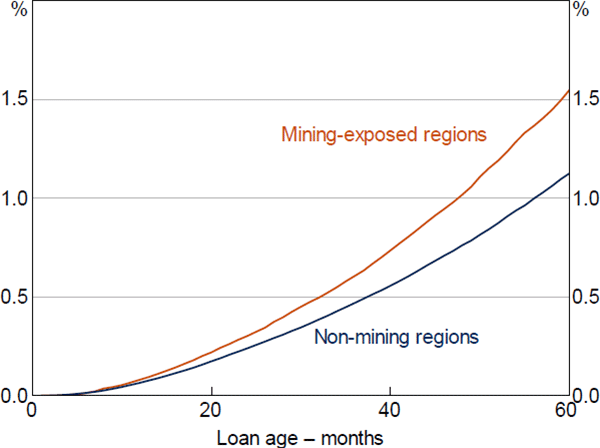
Sources: ABS; Author's calculations; CoreLogic data; RBA; Securitisation System
8. Conclusion and Policy Implications
This paper uses a new two-stage hazard modelling strategy to investigate the determinants of mortgage defaults in Australia and finds some evidence to support the double-trigger hypothesis. The main drivers of entries to arrears are ability-to-pay shocks, such as unemployment, while prepayment buffers reduce the probability that an ability-to-pay shock causes a borrower to enter arrears. The extent of negative equity is strongly correlated with whether a loan in arrears transitions to foreclosure.
From a policymaker's perspective, these estimates provide some clarity around the risks in the Australian mortgage market and the relative importance of ability-to-pay and equity factors for mortgage default. Since unemployment spells and reductions to income appear to be the key macroeconomic drivers of arrears, the unemployment rate and net income should be considered key variables when evaluating financial stability risks and in setting stabilising macroeconomic policy. Results regarding riskier loan characteristics and debt serviceability ratios may also have implications for lending standards policies, although this paper cannot provide policy recommendations as it does not consider the costs and benefits of changing lending standards. The main role played by housing prices is in loan losses given default, where a borrower already facing an ability-to-pay shock becomes more likely to enter foreclosure if they have negative equity. Prolonged periods of negative equity may in themselves also increase foreclosures as borrowers face a baseline probability of experiencing an idiosyncratic shock (such as illness). While this suggests that policies aimed at lowering LVRs at origination can be useful in reducing the probability that borrowers experience negative equity and thereby lower the risk of foreclosures, this must also be weighed against the costs of tightening credit supply – which is left to further research. Overall, the results in this paper imply that policies that promote a low unemployment rate and stable macroeconomic environment play a critical role in lowering the rate of mortgage defaults.
Appendix A : Summary Statistics and Variable Definitions
| First-stage sample(a) | Second-stage sample(b) | ||||||
|---|---|---|---|---|---|---|---|
| All loans | Entered arrears | Repaid | All loans | Foreclosure | Cured or repaid | ||
| Median loan balance | 335,600 | 355,900 | 337,300 | 296,100 | 299,500 | 293,200 | |
| Median indexed LVR(c) | 67 | 72 | 64 | 65 | 81 | 62 | |
| Negative equity (share)(c) | 3 | 7 | 1 | 7 | 26 | 4 | |
| Original LVR >80 (share) | 21 | 37 | 23 | 36 | 47 | 34 | |
| Median repayment-to-income ratio | 18 | 22 | 18 | 21 | 19 | 21 | |
| Median regional unemployment rate | 6 | 7 | 6 | 7 | 8 | 7 | |
| Mining region (share) | 13 | 26 | 10 | 28 | 57 | 24 | |
| Self-employed (share) | 17 | 22 | 16 | 25 | 28 | 25 | |
| Multiple debtors (share) | 66 | 55 | 67 | 57 | 49 | 58 | |
| Investor (share) | 32 | 28 | 31 | 26 | 38 | 24 | |
| IO (share) | 26 | 26 | 34 | 22 | 31 | 23 | |
| Full documentation (share) | 98 | 93 | 98 | 93 | 90 | 93 | |
| No of loans | 1,707,000 | 19,500 | 428,300 | 42,600 | 2,500 | 27,500 | |
|
Notes: (a) All loans originated in 2013 onwards; statistics measured at report date Sources: ABS; Author's calculations; CoreLogic data; RBA; Securitisation System |
|||||||
| Variable name | Variable definition | Unit | Sources |
|---|---|---|---|
| Indexed scheduled LVR | Scheduled balance / (most recent property valuation x SA3 region housing price index) | Loan | CoreLogic data; Securitisation System; Author's calculations |
| Debt serviceability ratio | Monthly loan repayments, estimated using credit foncier formulas / total borrower income at origination, indexed by state average weekly earnings | Loan | ABS; Securitisation System; Author's calculations |
| Loan type transitions | Calculated with six month lags of loan type and interest-only expiry date | Loan | Securitisation System; Author's calculations |
| Buffer | Maximum number of months of excess repayments, lagged 12 months | Loan | Securitisation System; Author's calculations |
| SEIFA | Index of Socio-economic Advantage and Disadvantage, using Census measures such as educational attainment | Postcode | ABS |
| Unemployment rate | SA3 region unemployment rate as at the 2016 Census for individuals that resided in the region as at the 2011 Census (to account for migration between SA3 regions) | SA3 region | ABS |
| Mining region | SA3 region with at least 3 per cent of employment in the mining industry or with at least two copper, iron ore or coal mines | SA3 region | ABS; Geoscience Australia; Author's calculations |
| Turnover ratio | Annual number of sales / estimated number of properties; trend | SA3 region | CoreLogic data; Author's calculations |
Definitions of additional variables from the Securitisation System are available at <https://www.rba.gov.au/mkt-operations/xls/consolidated-rmbs-reporting-guidance.xls>.
Appendix B : Full Results
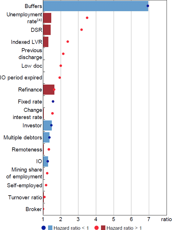
Notes:
Dots represent the relative hazard ratio of the 99th percentile observation to the 1st percentile; bars represent the interquartile range; hazard ratios that are less than 1 are inverted
(a) Estimate from model excluding the SEIFA variable
Sources: Sources: ABS; Author's calculations; CoreLogic data; RBA; Securitisation System
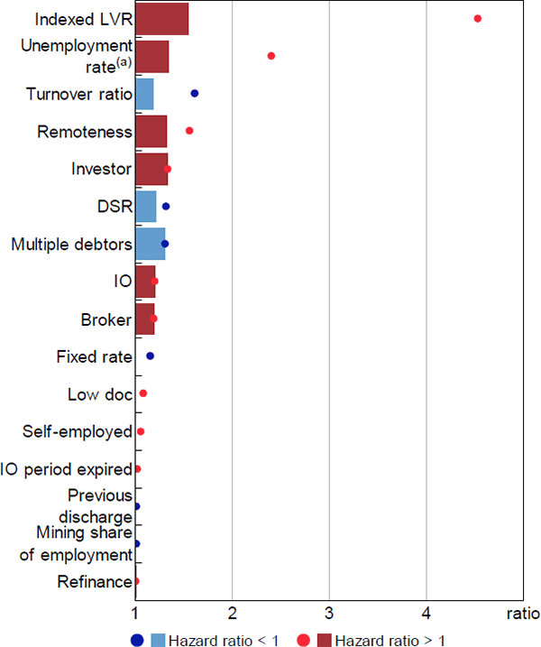
Notes:
Dots represent the relative hazard ratio of the 99th percentile observation to the 1st percentile; bars represent the interquartile range; hazard ratios that are less than 1 are inverted
(a) Estimate from model excluding the SEIFA variable
Sources: ABS; Author's calculations; CoreLogic data; RBA; Securitisation System
| Dependent variable: | Entered 90+ day arrears | Entered 90+ day arrears | Entered 90+ day arrears | Entered 90+ day arrears | Entered 90+ day arrears | Full repayment |
|---|---|---|---|---|---|---|
| Sample: | All loans | All loans | Non-mining | Mining-exposed | Negative equity | All loans |
| Model: | Base | Excl SEIFA | Base | Base | Base | Base |
| Indexed scheduled LVR (base = (60,70]) | ||||||
| (0,30] | 0.900* (0.045) |
0.882* (0.045) |
0.873* (0.050) |
1.068 (0.115) |
n/a | 0.834*** (0.008) |
| (30,40] | 0.779*** (0.045) |
0.769*** (0.045) |
0.763*** (0.049) |
0.854 (0.129) |
n/a | 0.787*** (0.008) |
| (40,50] | 0.827*** (0.035) |
0.820*** (0.035) |
0.813*** (0.037) |
0.926 (0.104) |
n/a | 0.830*** (0.006) |
| (50,60] | 0.885*** (0.027) |
0.881*** (0.027) |
0.885*** (0.029) |
0.906 (0.089) |
n/a | 0.918*** (0.005) |
| (70,80] | 1.142*** (0.023) |
1.145*** (0.023) |
1.167*** (0.025) |
0.954 (0.065) |
n/a | 0.989 (0.005) |
| (80,90] | 1.319*** (0.027) |
1.322*** (0.027) |
1.319*** (0.032) |
1.153* (0.061) |
n/a | 0.816*** (0.007) |
| (90,100] | 1.494*** (0.036) |
1.485*** (0.036) |
1.497*** (0.053) |
1.295*** (0.067) |
n/a | 0.556*** (0.012) |
| (100,110] | 1.872*** (0.046) |
1.841*** (0.046) |
1.745** (0.141) |
1.652*** (0.073) |
Base | 0.398*** (0.024) |
| (110,120] | 2.014*** (0.070) |
1.963*** (0.070) |
2.233** (0.270) |
1.737*** (0.093) |
1.019 (0.076) |
0.410*** (0.048) |
| (120,150] | 2.129*** (0.083) |
2.041*** (0.083) |
2.074* (0.260) |
1.750*** (0.105) |
1.006 (0.094) |
0.605** (0.048) |
| (150,200] | 2.730*** (0.145) |
2.623*** (0.145) |
n/a | 2.530*** (0.161) |
1.294 (0.160) |
0.670* (0.098) |
| 200+ | 3.299*** (0.201) |
3.233*** (0.201) |
n/a | 3.657*** (0.217) |
1.488* (0.230) |
0.652* (0.177) |
| Original LVR (base = (60,80]) | ||||||
| (0,60] | 1.054 (0.028) |
1.051 (0.028) |
1.093* (0.032) |
0.856* (0.062) |
0.767 (0.216) |
1.087*** (0.005) |
| 80+ | 1.286*** (0.019) |
1.307*** (0.019) |
1.312*** (0.023) |
1.241*** (0.038) |
1.415** (0.091) |
1.145*** (0.005) |
| Turnover ratio | 1.014 (0.007) |
1.020 (0.007) |
1.030* (0.007) |
0.934 (0.026) |
1.008 (0.040) |
1.041*** (0.001) |
| Unemployment rate | 1.075** (0.018) |
1.207*** (0.018) |
1.137 (0.042) |
1.150** (0.034) |
1.083 (0.073) |
1.061 (0.007) |
| Unemployment rate^2 | 0.998* (0.001) |
0.994** (0.001) |
0.992 (0.003) |
0.996* (0.002) |
1.000 (0.003) |
0.996 (0.000) |
| Serviceability ratio (base = (10,20]) | ||||||
| (0,10] | 0.605*** (0.030) |
0.618*** (0.030) |
0.586*** (0.036) |
0.659*** (0.055) |
0.550*** (0.112) |
1.016* (0.005) |
| (20,30] | 1.418*** (0.019) |
1.400*** (0.019) |
1.469*** (0.023) |
1.280*** (0.037) |
1.150 (0.075) |
1.008 (0.004) |
| (30,40] | 1.803*** (0.024) |
1.768*** (0.024) |
1.923*** (0.028) |
1.497*** (0.048) |
1.367** (0.101) |
0.988 (0.006) |
| 40+ | 1.926*** (0.033) |
1.883*** (0.033) |
2.015*** (0.039) |
1.731*** (0.064) |
1.550*** (0.145) |
0.934*** (0.009) |
| Lagged change in interest rates (bps; base = (–2,2]) | ||||||
| <–25 | 0.774*** (0.034) |
0.771*** (0.034) |
0.770*** (0.041) |
0.764*** (0.062) |
0.718* (0.125) |
0.801*** (0.008) |
| (–25,–2] | 0.933* (0.032) |
0.931* (0.032) |
0.923* (0.038) |
0.939 (0.059) |
0.782 (0.138) |
0.880*** (0.007) |
| (2,25] | 1.032 (0.021) |
1.032 (0.021) |
1.015 (0.025) |
1.076 (0.042) |
1.121 (0.081) |
0.893*** (0.005) |
| 25+ | 1.188*** (0.035) |
1.189*** (0.035) |
1.179*** (0.042) |
1.196** (0.065) |
1.233 (0.122) |
0.992 (0.007) |
| Repayment buffer (months; base = (1,6]) | ||||||
| <1 | 2.322*** (0.019) |
2.306*** (0.019) |
2.293*** (0.023) |
2.371*** (0.036) |
2.309*** (0.076) |
0.983** (0.004) |
| 6+ | 0.334*** (0.031) |
0.331*** (0.031) |
0.331*** (0.036) |
0.343*** (0.060) |
0.435*** (0.135) |
0.870*** (0.005) |
| Income <$180,000 | 0.931* (0.023) |
0.972 (0.023) |
0.926* (0.028) |
0.949 (0.045) |
0.840 (0.087) |
0.991 (0.004) |
| Loan type (base = principal and interest (P&I)) | ||||||
| IO | 0.786*** (0.020) |
0.771*** (0.020) |
0.760*** (0.024) |
0.869*** (0.039) |
1.033 (0.079) |
1.019*** (0.004) |
| Switched to IO | 2.831*** (0.067) |
2.778*** (0.067) |
2.954*** (0.084) |
2.538*** (0.112) |
2.244** (0.245) |
1.184*** (0.023) |
| Switched to P&I – IO period expired |
1.944*** (0.048) |
1.925*** (0.048) |
1.913*** (0.059) |
2.022*** (0.086) |
2.350*** (0.151) |
1.330*** (0.016) |
| Switched to P&I – voluntary | 0.298*** (0.190) |
0.293*** (0.190) |
0.279*** (0.225) |
0.360** (0.356) |
0.645 (0.508) |
0.880*** (0.025) |
| Investor | 0.674*** (0.019) |
0.681*** (0.019) |
0.653*** (0.022) |
0.739*** (0.037) |
0.728*** (0.075) |
0.915*** (0.004) |
| Self-employed | 1.185*** (0.020) |
1.188*** (0.020) |
1.179*** (0.024) |
1.199*** (0.041) |
1.284 (0.094) |
0.866*** (0.005) |
| Multiple debtors | 0.732*** (0.015) |
0.726*** (0.015) |
0.707*** (0.018) |
0.794*** (0.029) |
0.898 (0.062) |
1.086*** (0.003) |
| SEIFA | 0.998*** (0.000) |
n/a | 0.998*** (0.000) |
0.998*** (0.000) |
0.998 (0.001) |
1.000 (0.000) |
| Mining share of employment | 1.018*** (0.002) |
1.016** (0.002) |
1.046 (0.022) |
1.011 (0.003) |
1.015 (0.004) |
0.983*** (0.001) |
| Previous discharge | 2.149*** (0.036) |
2.165*** (0.036) |
2.181*** (0.041) |
2.039*** (0.075) |
2.481*** (0.172) |
1.250*** (0.012) |
| Low documentation | 2.013*** (0.042) |
2.008*** (0.042) |
2.058*** (0.047) |
1.869*** (0.088) |
2.133 (0.380) |
1.093*** (0.014) |
| Fixed rate | 0.635*** (0.024) |
0.637*** (0.024) |
0.636*** (0.027) |
0.637*** (0.047) |
0.609*** (0.093) |
0.574*** (0.005) |
| Loan purpose (base = purchase) | ||||||
| Construction | 1.070 (0.043) |
1.065 (0.043) |
1.268*** (0.051) |
0.720*** (0.083) |
0.787 (0.127) |
0.999 (0.010) |
| Further advance | 1.478*** (0.104) |
1.480*** (0.104) |
1.324* (0.132) |
1.785*** (0.167) |
2.577* (0.319) |
1.220*** (0.020) |
| Refinance | 1.636*** (0.016) |
1.639*** (0.016) |
1.699*** (0.019) |
1.464*** (0.031) |
1.434*** (0.065) |
1.185*** (0.003) |
| Broker-originated | 1.012 (0.016) |
1.010 (0.016) |
0.999 (0.019) |
1.045 (0.032) |
0.966 (0.067) |
0.992 (0.003) |
| Region (base = capital city) | ||||||
| Major city | 1.029 (0.030) |
1.083 (0.030) |
1.002 (0.034) |
0.910 (0.120) |
0.837 (0.533) |
1.006 (0.006) |
| Regional centre | 1.069 (0.024) |
1.156*** (0.024) |
1.010 (0.032) |
1.077 (0.056) |
1.071 (0.104) |
0.885*** (0.006) |
| Remote | 1.336*** (0.028) |
1.529*** (0.027) |
1.302*** (0.036) |
1.270* (0.064) |
1.279 (0.132) |
0.826*** (0.008) |
| State fixed effects | Yes | Yes | Yes | Yes | Yes | Yes |
| Time fixed effects | Yes | Yes | Yes | Yes | Yes | Yes |
| Deal and issuer type | Yes | Yes | Yes | Yes | Yes | Yes |
| No of observations | 12,370,383 | 12,370,842 | 10,442,510 | 1,927,873 | 216,898 | 12,370,383 |
| No of events | 19,625 | 19,626 | 14,350 | 5,275 | 1,236 | 427,589 |
| Concordance ratio | 0.787 | 0.786 | 0.784 | 0.775 | 0.736 | 0.634 |
|
Notes: ***, ** and * denote statistical significance at the 0.1, 1 and 5 per cent levels, respectively; standard errors are in parentheses Sources: ABS; Author's calculations; CoreLogic data; RBA; Securitisation System |
||||||
| Dependent variable: | Entered foreclosure | Entered foreclosure | Entered foreclosure | Entered foreclosure | Entered foreclosure | Cured | Full repayment |
|---|---|---|---|---|---|---|---|
| Sample: | All loans | All loans | Non-mining | Mining-exposed | Negative equity | All loans | All loans |
| Model: | Base | Excl SEIFA | Base | Base | Base | Base | Base |
| Indexed scheduled LVR (base = (60,70]) | |||||||
| (0,30] | 0.783 (0.127) | 0.785 (0.127) | 0.691* (0.168) | 0.941 (0.215) | n/a | 1.175*** (0.035) | 1.130* (0.048) |
| (30,40] | 0.761 (0.138) | 0.758 (0.138) | 0.554** (0.182) | 1.367 (0.221) | n/a | 1.151*** (0.035) | 1.024 (0.049) |
| (40,50] | 0.756* (0.118) | 0.756* (0.118) | 0.598** (0.149) | 1.204 (0.201) | n/a | 1.106** (0.031) | 1.095 (0.041) |
| (50,60] | 0.902 (0.101) | 0.901 (0.101) | 0.882 (0.118) | 0.921 (0.198) | n/a | 1.101** (0.028) | 1.000 (0.038) |
| (70,80] | 1.170 (0.084) | 1.171 (0.084) | 1.171 (0.103) | 1.198 (0.149) | n/a | 1.001 (0.026) | 0.922 (0.037) |
| (80,90] | 1.688*** (0.085) | 1.690*** (0.085) | 1.850*** (0.112) | 1.514** (0.143) | n/a | 0.967 (0.030) | 0.818*** (0.044) |
| (90,100] | 2.097*** (0.095) | 2.098*** (0.095) | 2.540*** (0.142) | 1.772*** (0.147) | n/a | 0.942 (0.040) | 0.679*** (0.063) |
| (100,110] | 2.515*** (0.107) | 2.509*** (0.107) | 3.919*** (0.196) | 2.068*** (0.156) | n/a | 0.807*** (0.054) | 0.471*** (0.098) |
| (110,120] | 3.261*** (0.130) | 3.248*** (0.130) | 5.011*** (0.326) | 2.698*** (0.174) | 1.321* (0.125) | 0.831* (0.086) | 0.687** (0.132) |
| (120,150] | 3.443*** (0.129) | 3.404*** (0.129) | 8.596*** (0.305) | 2.874*** (0.173) | 1.582** (0.126) | 0.818* (0.088) | 0.581* (0.151) |
| (150,200] | 4.604*** (0.155) | 4.535*** (0.155) | 1.970 (1.011) | 4.025*** (0.193) | 1.988*** (0.167) | 0.434*** (0.178) | 0.927 (0.201) |
| 200+ | 7.542*** (0.189) | 7.515*** (0.189) | n/a | 5.380*** (0.231) | 2.795*** (0.209) | 0.276*** (0.323) | 1.957*** (0.193) |
| Original LVR (base = (60,80]) | |||||||
| (0,60] | 0.923 (0.083) | 0.919 (0.083) | 0.956 (0.123) | 0.847 (0.116) | 0.849 (0.258) | 0.957 (0.025) | 1.048 (0.034) |
| 80+ | 1.000 (0.052) | 1.002 (0.051) | 0.967 (0.078) | 1.045 (0.072) | 0.988 (0.120) | 0.945** (0.020) | 1.053 (0.028) |
| Turnover ratio | 0.921*** (0.019) | 0.924*** (0.019) | 0.902** (0.031) | 0.977 (0.042) | 1.040 (0.047) | 1.007 (0.007) | 1.074*** (0.010) |
| Unemployment rate | 1.104 (0.050) | 1.128* (0.048) | 0.831 (0.142) | 1.183* (0.076) | 1.036 (0.124) | 0.996 (0.019) | 0.927* (0.032) |
| Unemployment rate^2 | 0.998 (0.003) | 0.997 (0.003) | 1.015 (0.009) | 0.994 (0.004) | 1.000 (0.006) | 1.001 (0.001) | 1.003 (0.002) |
| Serviceability ratio (base = (10,20]) | |||||||
| (0,10] | 1.172 (0.085) | 1.179 (0.085) | 1.317 (0.132) | 1.151 (0.112) | 1.042 (0.184) | 1.097* (0.036) | 0.987 (0.051) |
| (20,30] | 0.828* (0.065) | 0.823* (0.065) | 0.786* (0.096) | 0.869 (0.090) | 1.036 (0.140) | 0.985 (0.023) | 1.030 (0.033) |
| (30,40] | 0.817 (0.089) | 0.814* (0.089) | 0.753* (0.128) | 0.887 (0.127) | 1.141 (0.192) | 0.994 (0.031) | 1.100* (0.043) |
| 40+ | 0.891 (0.112) | 0.881 (0.111) | 0.969 (0.172) | 0.912 (0.148) | 1.178 (0.239) | 0.988 (0.043) | 0.962 (0.061) |
| Income <$180,000 | 0.890 (0.075) | 0.901 (0.074) | 0.825 (0.121) | 0.900 (0.097) | 0.675 (0.141) | 1.083* (0.031) | 0.940 (0.041) |
| Loan type (base =P&I) | |||||||
| IO | 1.198** (0.055) | 1.193** (0.055) | 1.068 (0.086) | 1.286** (0.074) | 1.201 (0.110) | 1.081** (0.021) | 1.012 (0.031) |
| Switched to P&I – IO period expired | 1.026 (0.095) | 1.025 (0.095) | 0.817 (0.165) | 1.121 (0.118) | 0.863 (0.164) | 1.001 (0.038) | 1.109 (0.051) |
| Investor | 1.334*** (0.050) | 1.337*** (0.050) | 1.481*** (0.074) | 1.219* (0.070) | 1.235 (0.108) | 1.000 (0.020) | 1.096** (0.027) |
| Self-employed | 1.062 (0.054) | 1.059 (0.054) | 1.112 (0.079) | 0.990 (0.076) | 0.924 (0.122) | 0.990 (0.019) | 1.151*** (0.026) |
| Multiple debtors | 0.766*** (0.043) | 0.766*** (0.043) | 0.641*** (0.064) | 0.889 (0.058) | 1.430*** (0.093) | 1.041* (0.015) | 1.152*** (0.022) |
| SEIFA | 0.999 (0.000) | n/a | 0.999 (0.001) | 0.999 (0.001) | 1.000 (0.001) | 1.001*** (0.000) | 1.001*** (0.000) |
| Mining share of employment | 1.000 (0.003) | 0.999 (0.003) | 0.901 (0.076) | 1.004 (0.004) | 0.993 (0.006) | 0.995 (0.002) | 0.992 (0.004) |
| Previous discharge | 0.983 (0.127) | 0.984 (0.127) | 1.235 (0.157) | 0.627* (0.226) | 0.710 (0.434) | 0.709*** (0.051) | 0.931 (0.064) |
| Restructuring arrangements | 0.364*** (0.084) | 0.363*** (0.084) | 0.336*** (0.120) | 0.388*** (0.121) | 0.554** (0.184) | 1.190*** (0.022) | 0.860*** (0.032) |
| Low documentation | 1.083 (0.099) | 1.077 (0.099) | 1.000 (0.134) | 1.193 (0.149) | 1.448 (0.352) | 0.768*** (0.038) | 0.891 (0.049) |
| Fixed rate | 0.864 (0.084) | 0.863 (0.084) | 0.853 (0.126) | 0.885 (0.113) | 0.794 (0.178) | 1.016 (0.027) | 0.849*** (0.041) |
| Loan purpose (base = purchase) | |||||||
| Construction | 1.145 (0.100) | 1.142 (0.100) | 1.556** (0.140) | 0.919 (0.145) | 0.850 (0.206) | 0.896** (0.042) | 0.857** (0.062) |
| Further advance | 0.793 (0.243) | 0.791 (0.243) | 0.531 (0.455) | 0.876 (0.294) | 0.826 (0.425) | 0.902 (0.076) | 1.033 (0.094) |
| Refinance | 1.007 (0.047) | 1.007 (0.047) | 1.088 (0.070) | 0.946 (0.065) | 0.931 (0.106) | 1.001 (0.017) | 1.039 (0.024) |
| Broker-originated | 1.192** (0.047) | 1.192** (0.047) | 1.216* (0.070) | 1.183* (0.064) | 1.124 (0.098) | 1.058** (0.016) | 0.791*** (0.024) |
| Region (base = capital city) | |||||||
| Major city | 1.325* (0.107) | 1.330* (0.107) | 1.401* (0.118) | 1.644 (0.419) | 0.696 (0.801) | 0.986 (0.032) | 0.939 (0.042) |
| Regional centre | 1.568*** (0.061) | 1.588*** (0.060) | 1.280* (0.102) | 1.714*** (0.105) | 1.675** (0.179) | 1.038 (0.024) | 0.941 (0.035) |
| Remote | 1.556*** (0.073) | 1.618*** (0.068) | 1.757*** (0.105) | 1.501** (0.127) | 1.386 (0.215) | 1.040 (0.027) | 0.742*** (0.043) |
| State fixed effects | Yes | Yes | Yes | Yes | Yes | Yes | Yes |
| Origination year fixed effects | Yes | Yes | Yes | Yes | Yes | Yes | Yes |
| Time fixed effects | Yes | Yes | Yes | Yes | Yes | Yes | Yes |
| Deal and issuer type | Yes | Yes | Yes | Yes | Yes | Yes | Yes |
| No of observations | 42,136 | 42,141 | 30,401 | 11,735 | 2,796 | 42,136 | 42,136 |
| No of events | 2,388 | 2,389 | 1,092 | 1,296 | 572 | 18,187 | 9,016 |
| Concordance ratio | 0.791 | 0.791 | 0.787 | 0.756 | 0.732 | 0.579 | 0.634 |
|
Notes: ***, ** and * denote statistical significance at the 0.1, 1 and 5 per cent levels, respectively; standard errors are in parentheses Sources: ABS; Author's calculations; CoreLogic data; RBA; Securitisation System |
|||||||
Appendix C : Robustness Checks – Multinomial Logit Models
The first-stage multinomial logit model shares many similarities with the competing risks, proportional hazards model, including producing similar results. The categories for dependent variable are entries to 90+ day arrears and full repayment, relative to the base category of remaining current on payments. It is estimated using quarterly observations for the same sample of loans and includes the same explanatory variables, plus seasoning (specified with a cubic term) as an explanatory variable.
The second-stage multinomial logit model differs more substantively to the baseline model. The dependent variable is each loan's status 12 months after entering arrears; the categories are foreclosure, curing and repayment, relative to the base category of remaining in arrears. Nonetheless, results are also similar to the proportional hazards model.
| Dependent variable: | Entered 90+ day arrears | Full repayment | Entered foreclosure | Cured | Full repayment |
|---|---|---|---|---|---|
| Model stage: | One | One | Two | Two | Two |
| Indexed scheduled LVR (base = (50,60]) | |||||
| (0,30] | 0.943 (−1.18) |
0.885*** (−8.60) |
0.929 (−0.49) |
1.189* (−2.41) |
1.194* (−2.02) |
| (30,40] | 0.813*** (−3.99) |
0.830*** (−16.28) |
0.826 (−1.15) |
1.181* (−2.39) |
1.099 (−1.13) |
| (40,50] | 0.860*** (−4.02) |
0.870*** (−13.94) |
0.803 (−1.39) |
1.074 (−1.18) |
1.075 (−1.06) |
| (60,70] | 0.904*** (−3.39) |
0.945*** (−7.43) |
0.786 (−1.92) |
1.067 (−1.04) |
1.023 (−0.36) |
| (70,80] | 1.110*** (−3.67) |
0.950*** (−6.05) |
1.006 (−0.07) |
0.905 (−1.83) |
0.855** (−2.61) |
| (80,90] | 1.253*** (−7.20) |
0.761*** (−25.35) |
1.529*** (−4.30) |
0.914 (−1.49) |
0.808** (−2.73) |
| (90,100] | 1.407*** (−8.13) |
0.512*** (−32.39) |
1.980*** (−5.24) |
0.912 (−1.07) |
0.633*** (−4.16) |
| (100,110] | 1.794*** (−9.95) |
0.377*** (−20.90) |
1.939*** (−4.40) |
0.667** (−3.29) |
0.399*** (−6.32) |
| (110,120] | 1.976*** (−9.14) |
0.396*** (−9.33) |
3.956*** (−5.47) |
0.954 (−0.23) |
0.763 (−1.02) |
| (120,150] | 2.117*** (−4.76) |
0.591** (−3.12) |
3.260*** (−4.52) |
0.754 (−1.32) |
0.602 (−1.62) |
| (150,200] | 2.696*** (−3.89) |
0.654** (−2.63) |
5.708*** (−5.26) |
0.558* (−2.04) |
1.077 (−0.17) |
| 200+ | 3.310*** (−7.70) |
0.637* (−2.37) |
6.135*** (−7.59) |
0.338** (−2.65) |
2.052** (−2.83) |
| Original LVR (base = (0,60]) | |||||
| (60,80] | 1.013 (−0.37) |
1.035*** (−4.94) |
0.867 (−1.26) |
0.938 (−1.35) |
1.035 (−0.63) |
| 80+ | 1.339*** (−12.04) |
1.219*** (−22.40) |
1.073 (−1.04) |
0.946 (−1.37) |
1.076 (−1.44) |
| Turnover ratio | 1.014 (−0.97) |
1.042*** (−8.01) |
0.897*** (−3.59) |
1.028* (−2.05) |
1.090*** (−4.52) |
| Unemployment rate | 1.078** (−2.95) |
1.060 (−1.58) |
1.083 (−0.98) |
0.963 (−1.24) |
0.921* (−2.02) |
| Unemployment rate^2 | 0.998* (−2.16) |
0.996 (−1.57) |
0.998 (−0.37) |
1.003 (−1.89) |
1.003 (−1.39) |
| Serviceability ratio (base = (10,20]) | |||||
| (0,10] | 0.606*** (−14.19) |
1.018** (−2.61) |
1.385** (−2.81) |
1.175* (−2.36) |
1.076 (−0.83) |
| (20,30] | 1.413*** (−13.35) |
1.003 (−0.46) |
0.869 (−1.52) |
1.001 (−0.02) |
1.058 (−1.17) |
| (30,40] | 1.789*** (−18.06) |
0.975** (−2.88) |
0.857 (−1.27) |
1.025 (−0.39) |
1.124 (−1.70) |
| 40+ | 1.922*** (−15.91) |
0.928*** (−5.51) |
0.994 (−0.04) |
0.980 (−0.23) |
0.988 (−0.12) |
| Lagged change in interest rates (bps; base = (−2,2]) | |||||
| <−25 | 0.781*** (−7.91) |
0.807*** (−23.77) |
n/a | n/a | n/a |
| (−25,−2] | 0.934* (−1.99) |
0.873*** (−17.30) |
n/a | n/a | n/a |
| (2,25] | 1.027 (−1.11) |
0.893*** (−17.23) |
n/a | n/a | n/a |
| 25+ | 1.185*** (−4.69) |
0.990 (−0.98) |
n/a | n/a | n/a |
| Repayment buffer (months; base = (1,6]) | |||||
| <1 | 2.315*** (−34.96) |
0.975*** (−4.44) |
n/a | n/a | n/a |
| 6+ | 0.335*** (−31.31) |
0.869*** (−19.69) |
n/a | n/a | n/a |
| Income <$180,000 | 0.931* (−2.57) |
0.990 (−1.43) |
0.799 (−1.90) |
1.036 (−0.58) |
0.889 (−1.63) |
| Loan type (base = P&I) | |||||
| IO | 0.798*** (−9.98) |
1.039*** (−7.06) |
1.265* (−2.43) |
1.142** (−3.06) |
1.022 (−0.44) |
| Switched to IO | 2.885*** (−13.88) |
1.195*** (−5.72) |
n/a | n/a | n/a |
| Switched to P&I – IO period expired | 2.008** (−14.33) |
1.387*** (−17.32) |
1.096 (−0.78) |
0.996 (−0.05) |
1.131 (−1.58) |
| Switched to P&I – voluntary | 0.298*** (−6.01) |
0.881*** (−4.11) |
n/a | n/a | n/a |
| Investor | 0.676*** (−16.51) |
0.918*** (−10.32) |
1.277** (−3.02) |
0.994 (−0.14) |
1.110* (−2.31) |
| Self-employed | 1.181*** (−6.77) |
0.862*** (−25.77) |
1.183* (−2.04) |
1.060 (−1.57) |
1.232*** (−4.93) |
| Multiple debtors | 0.730*** (−16.28) |
1.081*** (−14.73) |
0.876* (−2.24) |
1.084* (−2.53) |
1.231*** (−5.13) |
| SEIFA | 0.998*** (−8.17) |
1.000 (−0.78) |
1.000 (−0.48) |
1.002*** (−5.47) |
1.002*** (−4.34) |
| Mining share of employment | 1.018*** (−3.46) |
0.984*** (−6.74) |
0.996 (−0.87) |
0.990 (−1.87) |
0.982** (−2.75) |
| Previous discharge | 2.198*** (−19.64) |
1.280*** (−16.83) |
0.791 (−1.41) |
0.591*** (−5.71) |
0.727** (−2.89) |
| Restructuring arrangements | n/a | n/a | 0.497*** (−5.81) |
1.464*** (−7.40) |
1.144* (−2.39) |
| Low documentation | 2.040*** (−13.95) |
1.099*** (−4.96) |
0.731* (−1.98) |
0.574*** (−7.98) |
0.659*** (−4.67) |
| Fixed rate | 0.625*** (−19.95) |
0.562*** (−87.48) |
0.862 (−1.31) |
0.971 (−0.57) |
0.807*** (−3.49) |
| Loan purpose (base = purchase) | |||||
| Construction | 1.083 (−1.47) |
1.019 (−0.98) |
1.053 (−0.44) |
0.795** (−3.29) |
0.718*** (−3.94) |
| Further advance | 1.491*** (−3.77) |
1.235*** (−9.39) |
0.733 (−1.26) |
0.873 (−1.01) |
0.938 (−0.41) |
| Refinance | 1.635*** (−24.12) |
1.175*** (−32.20) |
0.972 (−0.39) |
0.997 (−0.10) |
1.055 (−1.39) |
| Broker-originated | 1.009 (−0.47) |
0.985* (−2.48) |
1.266*** (−3.62) |
1.100** (−2.90) |
0.812*** (−4.99) |
| Region (base = capital city) | |||||
| Major city | 1.026 (−0.51) |
1.003 (−0.14) |
1.338 (−1.61) |
0.984 (−0.20) |
0.944 (−0.60) |
| Regional centre | 1.079 (−1.72) |
0.894*** (−6.82) |
1.681*** (−5.77) |
1.105* (−2.24) |
1.008 (−0.13) |
| Remote | 1.344*** (−6.66) |
0.831*** (−12.37) |
1.731*** (−6.03) |
1.127* (−2.37) |
0.792*** (−3.42) |
| Seasoning | 1.112*** (−19.53) |
1.067*** (−46.86) |
n/a | n/a | n/a |
| Seasoning^2 | 0.998*** (−14.01) |
0.999*** (−32.20) |
n/a | n/a | n/a |
| Seasoning^3 | 1.000*** (−11.83) |
1.000*** (−23.45) |
n/a | n/a | n/a |
| State fixed effects | Yes | Yes | Yes | Yes | Yes |
| Origination year fixed effects | No | No | Yes | Yes | Yes |
| Time fixed effects | Yes | Yes | Yes | Yes | Yes |
| Deal and issuer type | Yes | Yes | Yes | Yes | Yes |
| No of observations | 12,370,838 | 12,370,838 | 32,816 | 32,816 | 32,816 |
| No of events | 18,035 | 442,496 | 1,870 | 15,290 | 7,720 |
| Pseudo R2 | 0.041 | 0.041 | 0.057 | 0.057 | 0.057 |
|
Notes: ***, ** and * denote statistical significance at the 0.1, 1 and 5 per cent levels, respectively; standard errors are in parentheses Sources: ABS; Author's calculations; CoreLogic data; RBA; Securitisation System |
|||||
References
Adelino M, K Gerardi and PS Willen (2013), ‘Why Don't Lenders Renegotiate More Home Mortgages? Redefaults, Self-Cures and Securitization’, Journal of Monetary Economics, 60(7), pp 835–853.
Albanesi S, G De Giorgi and J Nosal (2017), ‘Credit Growth and the Financial Crisis: A New Narrative’, NBER Working Paper No 23740.
Ambrose BW and CA Capone (1998), ‘Modeling the Conditional Probability of Foreclosure in the Context of Single-Family Mortgage Default Resolutions’, Real Estate Economics, 26(3), pp 391–429.
ASIC (Australian Securities and Investment Commission) (nd), ‘Problems Paying Your Mortgage’, viewed 25 February 2020. Available at <https://moneysmart.gov.au/home-loans/problems-paying-your-mortgage>.
Bajari P, CS Chu and M Park (2008), ‘An Empirical Model of Subprime Mortgage Default from 2000 to 2007’, NBER Working Paper No 14625.
Berry M, T Dalton and A Nelson (2010), Mortgage Default in Australia: Nature, Causes and Social and Economic Impacts, AHURI Final Report No 145, Australian Housing and Urban Research Institute, Melbourne.
Bhutta N, J Dokko and H Shan (2017), ‘Consumer Ruthlessness and Mortgage Default during the 2007 to 2009 Housing Bust’, The Journal of Finance, 72(6), pp 2433–2466.
Cox D (1972), ‘Regression Models and Life-Tables’, Journal of the Royal Statistical Society. Series B (Methodological), 34(2), pp 187–202.
Deng Y, JM Quigley and R Van Order (2000), ‘Mortgage Terminations, Heterogeneity and the Exercise of Mortgage Options’, Econometrica, 68(2), pp 275–307.
Deng Y, JM Quigley, R Van Order and Freddie Mac (Federal Home Loan Mortgage Corporation) (1996), ‘Mortgage Default and Low Downpayment Loans: The Costs of Public Subsidy’, Regional Science and Urban Economics, 26(3–4), pp 263–285.
Disney R and J Gathergood (2013), ‘Financial Literacy and Consumer Credit Portfolios’, Journal of Banking & Finance, 37(7), pp 2246–2254.
Do HX, D Rösch and H Scheule (2020), ‘Liquidity Constraints, Home Equity and Residential Mortgage Losses’, The Journal of Real Estate Finance and Economics, 61(2), pp 208–246.
Elul R, NS Souleles, S Chomsisengphet, D Glennon and R Hunt (2010), ‘What “Triggers” Mortgage Default?’, The American Economic Review, 100(2), pp 490–494.
Fernandes K and D Jones (2018), ‘The Reserve Bank's Securitisation Dataset’, RBA Bulletin, December, viewed 19 February 2020. Available at <https://www.rba.gov.au/publications/bulletin/2018/dec/the-reserve-banks-securitisation-dataset.html>.
Fine JP and RJ Gray (1999), ‘A Proportional Hazards Model for the Subdistribution of a Competing Risk’, Journal of the American Statistical Association, 94(446), pp 496–509.
Foote CL and PS Willen (2017), ‘Mortgage-Default Research and the Recent Foreclosure Crisis’, Federal Reserve Bank of Boston Research Department Working Paper No 17-13.
Foster C and R Van Order (1984), ‘An Option-Based Model of Mortgage Default’, Housing Finance Review, 3(4), pp 351–372.
Gerardi K, KF Herkenhoff, LE Ohanian and PS Willen (2018), ‘Can't Pay or Won't Pay? Unemployment, Negative Equity, and Strategic Default’, The Review of Financial Studies, 31(3), pp 1098–1131.
Gerardi K, A Lehnert, SM Sherlund and PS Willen (2008), ‘Making Sense of the Subprime Crisis’, Brookings Papers on Economic Activity, Fall, pp 69–145.
Ghent AC and M Kudlyak (2011), ‘Recourse and Residential Mortgage Default: Evidence from US States’, The Review of Financial Studies, 24(9), pp 3139–3186.
Guiso L, P Sapienza and L Zingales (2013), ‘The Determinants of Attitudes toward Strategic Default on Mortgages’, The Journal of Finance, 68(4), pp 1473–1515.
Gyourko J and J Tracy (2014), ‘Reconciling Theory and Empirics on the Role of Unemployment in Mortgage Default’, Journal of Urban Economics, 80, pp 87–96.
Kau JB, DC Keenan and T Kim (1994), ‘Default Probabilities for Mortgages’, Journal of Urban Economics, 35(3), pp 278–296.
Kearns J (2019), ‘Understanding Rising Housing Loan Arrears’, Keynote address to the 2019 Property Leaders' Summit, Canberra, 18 June.
Kent C (2017), ‘Some Innovative Mortgage Data’, Address given to Moody's Analytics Australia Conference 2017, Sydney, 14 August.
Kent C (2018), ‘The Limits of Interest-Only Lending’, Address to the Housing Industry Association Breakfast, Sydney, 24 April.
Kohler M (2017), ‘Mortgage Insights from Securitisation Data’, Address to the Australian Securitisation Forum, Sydney, 20 November.
Kruger S (2018), ‘The Effect of Mortgage Securitization on Foreclosure and Modification’, Journal of Financial Economics, 129(3), pp 586–607.
Linn A and RC Lyons (2019), ‘Three Triggers? Negative Equity, Income Shocks and Institutions as Determinants of Mortgage Default’, Bank of England Staff Working Paper No 812.
Mian A, A Sufi and F Trebbi (2015), ‘Foreclosures, House Prices, and the Real Economy’, The Journal of Finance, 70(6), pp 2587–2634.
Mincer J (1991), ‘Education and Unemployment’, NBER Working Paper No 3838.
Piskorski T, A Seru and V Vig (2010), ‘Securitization and Distressed Loan Renegotiation: Evidence from the Subprime Mortgage Crisis’, Journal of Financial Economics, 97(3), pp 369–397.
RBA (Reserve Bank of Australia) (2018), ‘Assessing the Effects of Housing Lending Policy Measures’, Financial Stability Review, October, pp 75–88.
RBA (2019), ‘Box B: Housing Price Falls and Negative Equity’, Financial Stability Review, April, pp 34–37.
Read M, C Stewart and G La Cava (2014), ‘Mortgage-Related Financial Difficulties: Evidence from Australian Micro-Level Data’, RBA Research Discussion Paper No 2014–13.
Copyright and Disclaimer Notice
CoreLogic Disclaimer
The following Disclaimer Notice applies to content that uses data from CoreLogic:
This publication contains data, analytics, statistics, results and other information licensed to us by RP Data Pty Ltd trading as CoreLogic Asia Pacific (CoreLogic Data).
© Copyright 2020. RP Data Pty Ltd trading as CoreLogic Asia Pacific (CoreLogic) and its licensors are the sole and exclusive owners of all rights, title and interest (including intellectual property rights) subsisting in the CoreLogic Data reproduced in this publication. All rights reserved.
The CoreLogic Data provided in this publication is of a general nature and should not be construed as specific advice or relied upon in lieu of appropriate professional advice.
While CoreLogic uses commercially reasonable efforts to ensure the CoreLogic Data is current, CoreLogic does not warrant the accuracy, currency or completeness of the CoreLogic Data and to the full extent permitted by law excludes all loss or damage howsoever arising (including through negligence) in connection with the CoreLogic Data.
Acknowledgements
I would like to thank Leon Berkelmans, James Bishop, Anthony Brassil, Bernadette Donovan, Nicholas Garvin, Jonathan Kearns, Gianni La Cava, Harald Scheule, John Simon, Michelle Wright and seminar participants at the Reserve Bank of Australia for useful discussions and feedback. The views expressed in this paper are those of the author and do not necessarily reflect the views of the Reserve Bank of Australia. The author is solely responsible for any errors.
Footnotes
There are some exceptions. Elul et al (2010) use borrowers' credit card data as a proxy for liquidity constraints. Gerardi et al (2018) highlight the importance of unemployment and disability shocks using household-level survey data. [1]
Self-securitisations are held entirely by the originating banks for use as collateral in the RBA's market operations. Many of these deals have ‘open’, or ‘revolving’, pools; that is, loans can be added or removed from the pool. [2]
The scheduled loan balance differs from the current loan balance by abstracting from any additional repayments previously made, including those in redraw and offset accounts, which a borrower would be able to draw upon prior to defaulting. The calculation does not take into account additional debts, such as credit card debts or debts with other lenders. [3]
This figure is higher than estimates in RBA (2019) due to the use of scheduled balances in the LVR calculation. Estimates from the Securitisation Dataset may understate the incidence of negative equity due to the skew towards loans with lower LVRs at origination, or overstate it due to the prevalence of newer loans in the dataset. [4]
Using the unadjusted unemployment rate in my model produced smaller coefficients that were generally not statistically significant.[5]
This figure is based on the indexed LVR at the point of entering arrears; results are little changed after accounting for subsequent changes to housing prices. It is possible that borrowers with substantial negative equity may still choose to cure if they expect housing prices to subsequently recover. [6]
This may also reflect loans entering foreclosure in the same reporting month as entering 90+ day arrears or definitional differences of what constitutes 90+ days (i.e. whether this is based on time or balance in arrears). [7]
The difficulty in interpretation stems from variables which are positively correlated with the competing risk appearing to have a preventative effect against the event of interest – since the individual is less likely to be in the risk set – even when those variables are in fact uncorrelated with the event of interest directly. See Fine and Gray (1999) for an implementation. [8]
To check the robustness of my results, I estimate a multinomial logit model that does not treat the competing risks as independent. See Appendix C for results. [9]
Loans may also be removed from the dataset when a marketed RMBS deal is called, or when collateral is substituted out of a self-securitisation. [10]
The dataset begins in 2015; estimates suggest that relatively few loans are refinanced within the first two years since origination, and very few loans enter arrears in the first two years. Loans originated in 2013 and 2014 coincided with the housing price peak in many mining-exposed regions and provide useful variation in equity that is needed for this analysis. [11]
See Cox (1972) for a discussion of why multiple observations must be used when the variable may be correlated with the time dimension. [12]
To investigate the determinants of the competing risks, I also estimate a separate model for each event. [13]
The region reported in the data is typically that of the property, rather than the borrower. These will be equivalent where the borrower is an owner-occupier, but may differ for investors.
Specifications using the change in the regional unemployment rate, rather than the level, were also tested. However, these data did not adjust for internal migration and the variable was found to have smaller effects in the models.
[14]Serviceability ratios are calculated as scheduled monthly loan repayments as a share of indexed income (income at origination, indexed by state average weekly earnings). [15]
Buffers are calculated as the number of months of scheduled repayments that the borrower has accumulated as excess repayments. As borrowers draw down on these buffers until they enter arrears, the maximum buffer up until 12 months prior to the estimation period is used to avoid bias in the estimated ‘protective’ effect of this variable. [16]
Appendix B also includes results for the competing risks, as well as models estimated over the subset of loans with negative equity and the subset of loans located in mining-exposed regions. Multinomial logit results, as a robustness check, can be found in Appendix C and are also broadly consistent with the results presented below. [17]
Models that include only the main variables of interest have concordance ratios around 0.75. Concordance ratios are approximately equal to the area under the ROC curve for Cox models. [18]
In general, multicollinearity should not be dealt with by excluding relevant variables (due to omitted variable bias). But I am using these variables as proxies for an ability-to-pay shock. So omitting the socio-economic index is fine as long as the regional unemployment rate effect is interpreted as a combination of the true effect and any correlated changes in the socio-economic index. [19]
This hazard ratio is from the model estimated without the socio-economic index. In the model with the socio-economic index, the regional unemployment hazard ratio is 1.08. [20]
The Socio-Economic Indexes for Areas (SEIFA) are constructed by the Australian Bureau of Statistics from Census indicators such as unemployment, educational attainment, English language proficiency and car ownership. I use the socio-economic indices of relative advantage and disadvantage, which are at the postcode level (a finer level of aggregation than other regional statistics used throughout this paper). [21]
This was largely in response to regulatory measures introduced by the Australian Prudential Regulation Authority on the share of lending to investors and for IO loans. [22]
In particular, many astute IO borrowers who were not liquidity constrained had already voluntarily switched to making principal repayments to avoid the increase in interest rates on IO loans (see also RBA (2018)). [23]
The magnitude of the DSR estimates is larger than is typically found in the international literature. [24]
Surprisingly, borrowers that had high incomes (defined as a combined indexed income above $180,000) were more likely to enter arrears, all else equal. [25]
Another possibility is that negative equity may reduce a borrower's ability to avoid arrears through full repayment, either by preventing a borrower with an unaffordable loan from refinancing or because the borrower may be reluctant to sell the property due to loss aversion. This is an example of the competing risk not being independent of the event of interest; negative equity reduces the probability of the borrower experiencing the competing risk and therefore indirectly increases the probability of experiencing the event of interest. The Cox model assumes that competing risks are independent and does not capture the increase in risk implied in this example. [26]
These results also hold when the model is estimated over the subset of loans with negative equity. [27]
Figures 15 and 16 include results for key variables only. Figures including controls can be found in Appendix B. [28]
An unexpectedly high share of loans in mining-exposed regions that were deeply in negative equity exited via full repayment, crystallising losses for borrowers. Perhaps these borrowers had other assets with positive equity, and wished to avoid foreclosure due to full recourse. [29]
Estimates use medians of continuous variables for the full subset of loans and categorical variables are set to the base/modal outcome. The baseline hazard is estimated using the Kalbfleisch-Prentice estimator (which reduces to the Kaplan-Meier estimate of the survival curve where coefficients are 0), post the estimation of the Cox model. [30]