Research Discussion Paper – RDP 2018-02 Affine Endeavour: Estimating a Joint Model of the Nominal and Real Term Structures of Interest Rates in Australia
February 2018
1. Introduction
Expectations of future nominal and real interest rates and inflation are crucial economic quantities. Expectations of nominal interest rates provide information about the expected path of monetary policy. Expectations for real interest rates, particularly a long way into the future, provide information about the economy's expected potential growth rate and the neutral real interest rate: the real rate that is expected to prevail in the medium term once all transitory shocks have dissipated.[1] In many economic models, monetary policy is deemed expansionary if current real rates are below this neutral rate, and contractionary if above. Finally, inflation expectations influence price- and wage-setting behaviour, and so affect observed inflation and economic outcomes more generally. Measures of expected inflation may also indicate if, and over what horizon, individuals believe that the central bank will meet its inflation target.
Nominal and inflation-indexed bond yields contain information about market participants' expectations for expected nominal and real rates, respectively. The difference between these two yields, referred to as break-even inflation, contains information about expected inflation. However, these yields also incorporate risk premia, which compensate investors for the various risks that they take on in buying a bond rather than investing in cash. This makes interpretation more difficult, as changes in yields could reflect changes in expectations or premia (or both).
One way to separate these premia from the ‘pure’ expectations component is to use an affine term structure model (ATSM). These models are widely used by policymakers and academics, and have been estimated for a broad range of countries for each of the above variables separately as well as jointly. Some key papers in the literature include: Duffie and Kan (1996), Dai and Singleton (2000) and Duffee (2002) who introduce and popularise the class of ATSMs that we work with; Kim and Orphanides (2012) who argue for the inclusion of survey data to increase the robustness of estimation, as well as Kim and Wright (2005) and Chernov and Mueller (2012) who also work with survey data; Joslin, Singleton and Zhu ((2011); hereafter referred to as JSZ), Hamilton and Wu (2012) and Adrian, Crump and Moench (2013) who introduce efficient estimation methods for these models; and Krippner (2013, 2015) who introduces a tractable framework for enforcing the zero lower bound on interest rates, which is particularly important to account for when the short-term nominal interest rate is near the lower bound, as has been the case in the United States, euro area and Japan recently (although not Australia).
In this paper we estimate a joint model of the term structures of nominal and real yields, which allows us to extract information on expected future short-term nominal and real interest rates, as well as inflation. The model is intended to be a ‘workhorse’ model that can be used for ongoing analysis. We take this into account in our modelling choices, and try to ensure that the model is parsimonious and relatively easy to update.
The results suggest that medium- to long-term expectations for the future short-term real interest rates, which some use as a measure of the neutral real interest rate, have declined somewhat over recent years. Meanwhile longer-term inflation expectations, having fallen over the 1990s as the Reserve Bank's inflation-targeting framework gained credibility, have been reasonably stable more recently, particularly compared with what is implied by break-even inflation rates. The results also suggest that a large portion of the decline in yields on Australian government securities (AGS) since the global financial crisis has reflected lower real term premia – the risk premium associated with variation in real interest rates – rather than declines in inflation expectations or inflation risk premia – premia associated with variation in inflation. The decline has mirrored that in US term premia, suggesting that it reflects some global factor such as foreign central banks' quantitative easing programs and the associated portfolio rebalancing flows.
As well as the Australia-specific contribution, our paper also contributes to the broader literature on ATSMs. Most notably, we extend the technique JSZ use to estimate a nominal ATSM so that we can estimate a joint model of nominal and real yields.[2] We also document how casting the model in terms of a Kalman filter and allowing the survey data to be fully exploited appears to aid estimation. This finding is somewhat counter to JSZ and Guimarães (2016), who find that filtering does not substantially change results. The difference likely reflects the fact that our zero-coupon real yield data contain a moderate amount of measurement error, given Australia has relatively few inflation-indexed bonds on issue, which makes filtering out the noise more important in our case. As such, the finding may be relevant for other countries with a limited number of inflation-indexed bonds, such as Germany and New Zealand. Finally, we also add to the literature by applying these ATSM techniques to an advanced economy that has not been subject to the effective lower bound for interest rates, unlike the United States, United Kingdom or euro area, which are more commonly examined in the literature.
2. The Model
We start by outlining the model that we will use in this paper. It is a joint model of the nominal and real term structures of interest rates. As has been well documented in the literature (e.g. JSZ; Guimarães 2016), there are a number of difficulties associated with the estimation of ATSMs, namely: small-sample problems, and numerical and computational issues. We address the first by incorporating survey data into the estimation, and address the latter by employing a generalised version of the JSZ normalisation. Below we discuss exactly how these are incorporated into the model. We work in discrete time throughout. For a more detailed treatment and derivation of the model, see Appendix A.
2.1 Deriving a Joint Affine Term Structure Model
The basic structure of ATSMs is relatively simple. These models assume that there are underlying (latent or observable) ‘pricing’ factors that drive both observable economic variables, such as the short-term interest rate or the inflation rate, and also risk preferences via a so-called ‘price of risk’. They are called affine models because they imply that observable bond yields are linear functions of these factors.
2.1.1 An ATSM of nominal interest rates
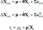
Considering first an ATSM of nominal interest rates, we assume that the one-period nominal interest rate (rt) is given by
where ρ0 is a scalar and ρ1 is a vector, so that rt is a linear function of the N pricing factors Xt. Moreover, we assume that the data-generating process (also called the ‘real-world distribution’ or ‘P dynamics’) of these pricing factors is a vector autoregressive (VAR) process with one lag
where μ is an N × 1 vector of intercepts, θ is an N × N matrix describing the evolution of Xt, and the N error terms εt + 1 ~N(0,IN).[3] Combining Equations (1) and (2) shows that the evolution of the short-term rate is controlled by the P dynamics.
As investors are risk averse, the price that they are willing to pay for a bond depends both on the expected level of interest rates over the life of the bond (governed by Equations (1) and (2)) and the risk that owning a bond entails, relative to rolling funds in short-dated securities. Following Duffee (2002), we assume that the market price of risk is also a linear function of the factors and is given by
where λt is an N × 1 vector that represents the price of risk associated with each of the factors at time t, λ0 is an N × 1 vector and λ1 is an N × N matrix. The specification implies that for each factor i, the compensation demanded by investors for bearing the risk associated with that factor is a constant λ0,i plus a linear combination of all the factors.
The market price of risk in turn determines the term premium, which is the compensation that investors receive/pay for locking in an interest rate for a long period, rather than rolling over short-dated securities. As discussed in Cochrane (2001), the size and sign of this premium will depend on two things:
- The amount of risk in the economy (i.e. the volatility/uncertainty around the future path of interest rates and the level of consumption).
- The covariance between bond returns and agents' marginal utility of consumption in different states of the world. That is, whether the bond provides a hedge for consumption risk or adds to consumption risk. If the bond is expected to provide relatively high returns during bad economic times when consumption is low and the marginal utility of additional consumption is high, then the bond provides a hedge to agents' consumption risk. In this case, owning bonds is similar to owning insurance against bad states of the world. Similar to normal insurance contracts, agents will be willing to pay extra for this hedge and so the bond yield, which is inversely related to its price, will be below the average interest rate expected to prevail over the life of the bond, resulting in a negative term premium. If, on the other hand, the bond is expected to fall in value during bad economic times, then it adds to investors' risk and investors will demand a higher yield, and therefore pay a lower price, resulting in a positive term premium.[4]
If we impose a no-arbitrage condition and assume a particular functional form for how agents price risk (called the ‘stochastic discount factor’), Equations (1) to (3) imply a set of pricing equations for zero-coupon nominal bond yields. In particular,
where  is the yield at time t for an n-period zero-coupon nominal bond (i.e. a bond that matures in n periods), and An and Bn are functions of the underlying model parameters (see Appendix A for further details). Of note, these bond pricing equations turn out to be equivalent to what would be obtained by assuming that investors were risk neutral (so λ0 = 0 and λ1 = 0) but that the pricing factors followed some other risk-adjusted (or risk-neutral) dynamics, often referred to as the ‘Q dynamics’
for  and
and  . In the literature μ and θ are often referred to as ‘P parameters’ as they determine the real-world or P dynamics, while
  and
and  , or equivalently, λ0 and λ1, are referred to as ‘Q parameters’.
2.1.2 An ATSM of real interest rates
Real zero-coupon bonds pay one unit of consumption good at time t + n, or Qt + n/Qt units of nominal value, where Qt is the price level at time t. This is in contrast to nominal zero-coupon bonds, which pay one unit of nominal income at time t + n.
We define the one-period inflation rate πt as
and, similar to the one-period nominal interest rate, assume it to be linear in the factors
Using the same assumptions as above (i.e. those regarding the P dynamics, the nominal rates, the price of risk, the functional form of the stochastic discount factor and the lack of arbitrage opportunities) leads to a similar set of pricing equations for real zero-coupon bonds, where
for  the real yield at time t for an n-period zero-coupon inflation-indexed bond, and
  and
and  functions of the underlying model parameters (including those for inflation).
2.1.3 Incorporating surveys
As noted above, the bond pricing equations are the same in the case where investors are risk neutral and the pricing factors follow the Q dynamics, and the case where investors are risk averse, but the pricing factors follow the ‘true’ P dynamics. In practical terms, this means that the cross-section of bond yields only identifies the Q dynamics. To separate out the P dynamics we have to rely on the time series of interest rates, which follow the true P dynamics.
The difficulty is that interest rates tend to be very persistent, and so even an apparently long sample (25 years) may only contain a small number of interest rate cycles, and only a small amount of information on the P dynamics. As such, ATSMs tend to be subject to small-sample problems.
For example, Bauer, Rudebusch and Wu (2012) note that the first step of the JSZ estimation procedure (discussed in more detail below) involves estimating a VAR on the observed pricing factors, which, having been constructed from the yield data, are highly persistent. VARs estimated using highly persistent series tend to produce downwardly biased estimates of the persistence of the series in small samples. As such, the approach will tend to underestimate the persistence of the observable factors and therefore produce estimates of long-term expected interest rates that are too stable.[5]
Two approaches have been suggested to address these small-sample issues. The first is to use statistical small-sample adjustments, such as bootstrapping, as proposed by Bauer et al (2012). The second is to incorporate surveys, as in Kim and Orphanides (2012). Guimarães (2016) argues that, as the issue fundamentally relates to a lack of information, the solution is to add more information on the P dynamics, and that this can be achieved by incorporating surveys as they provide additional cross-sections of expected future rates.[6] We follow the latter approach and incorporate survey data on interest rate and inflation expectations, which we treat as unbiased but noisy readings on the underlying quantities.[7] This can be done relatively easily. For example, the expected one-period inflation rate in n periods' time is given by
which can be solved in terms of the model parameters by iterating forward using Equation (2); see Appendix B.
2.2 The JSZ Normalisation
The ATSM described above is not identified unless we apply some normalisations. For intuition, consider a model that matches a set of observed yields and survey expectations. If we were to multiply the pricing factors and appropriate model parameters by negative one, the model would still fit the observables, but the parameters and pricing factors would be different.
Many papers follow Dai and Singleton (2000) in normalising the volatility matrix. This creates a strong link between the P and Q parameters because the volatility matrix appears in both the P and Q dynamics (Equations (2) and (5)), leading to an ill-behaved likelihood surface (i.e. one with multiple local maxima and flat areas), and therefore to computational difficulties, as these models are estimated by numerically maximising the likelihood function.
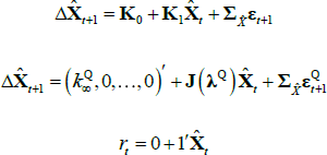
JSZ propose a different normalisation that largely breaks the link between the P and Q parameters, leading to a better-behaved likelihood function.[8] In particular, JSZ note that the nominal ATSM outlined above is observationally equivalent to another ATSM with a transformed state variable  that can be summarised as
where  is a scalar, J(λQ) is a diagonal matrix,
  is a lower triangular matrix and 1′ is a vector of ones. Moreover, JSZ show that if the original pricing factors (Xt) are taken to be some linear combination of the yields, such as the principal components, the normalisation delivers a complete bifurcation of the likelihoods of the P and Q dynamics. In this case one can estimate the P parameters by estimating a VAR on the observed factors using ordinary least squares (OLS). The remaining Q parameters can then be estimated by maximising the likelihood over the observed yields, conditional on the previously estimated P parameters. This significantly cuts down on the number of model parameters that must be estimated by numerical optimisation, and so makes estimation faster and more stable.
Extending this approach to account for real bonds is relatively simple. With the transformed state variable, the equation for inflation becomes
where the mapping between the parameters in Equations (6) and (9) is the same as the mapping between those in Equations (1) and (8). As such, we can simply add the recursive pricing equation for the real bonds to the Q optimisation and maximise the likelihood of the observed nominal and real yields, conditional on the P dynamics.
3. Data and Estimation
3.1 Estimation
As discussed in JSZ, maximising the model likelihood conditional on the observed factors imposes the assumption that the factors are ‘priced correctly’ – essentially, that there are no (or limited) measurement errors or breaches of no arbitrage conditions – but has the benefit of exploiting the JSZ technique to significantly speed up estimation. This is likely to be a reasonably strong assumption in our case given the limited number of inflation-linked bonds trading at any one time.
For this reason we use a two-step estimation procedure. First, we maximise the model likelihood conditional on the observed factors.[9] In doing so we cannot separately estimate the P dynamics in this first estimation step, as the modelled counterparts of the surveys rely on both the P parameters and some other parameters used to price bonds, such as the inflation parameters. Instead, we jointly maximise the likelihood function of the observed factors, the observed yields and the surveys (all the while holding the pricing factors fixed as the principal components of the relevant yield data). We use VAR estimates of the P parameters as starting points for this optimisation. The model is more difficult to estimate than in the standard JSZ set-up without survey data, but it is still simpler to estimate than earlier approaches as the dependency between the P and Q parameters remains relatively weak under the JSZ normalisation.
In the second step we relax the assumption that the factors are priced correctly by casting the model in terms of a Kalman filter and re-optimising using the parameter estimates from the first step as starting values.[10] Relaxing the assumption that the factors are priced correctly has two benefits: it allows us to model estimates of real zero-coupon yields as being noisy and/or observed with error, which, as discussed above, is useful given the limited number of inflation-linked bonds trading at any one time; and it allows the survey data to affect the factors, as they should. The Kalman filter also gives us scope to drop real zero-coupon yields from the model if there are no inflation-indexed bonds with similar maturities outstanding. Such data points are likely to be particularly noisy and relatively more dependent on the interpolation method employed, and so dropping them should increase the robustness of our estimates.[11]
The allowance for noise means that Equations (4) and (7) become
where  and
and  . We also allow for errors/uncertainty in the survey responses. Instead of calibrating the variance of these errors, we allow them to be estimated alongside the other parameters. This approach is more common in the literature and allows the data to ‘speak for itself’. We assume that the errors are independent, homoskedastic and normally distributed, and allow the error variances to differ for each type of forecast data that we use.
3.2 Data and Observable Factors
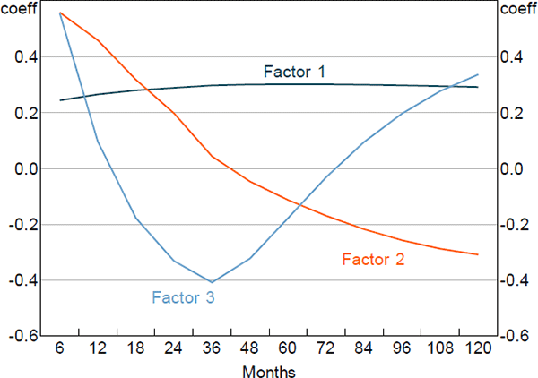
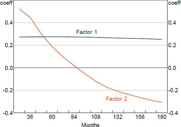
For the first stage of the estimation we need a set of observable factors that are linear functions of the yields. Consistent with Abrahams et al (2016) we use the first K principal components from a panel of nominal interest rates. We also use the first L principal components from a panel of real yields that have been orthogonalised with respect to the nominal factors by regressing the real yields on the nominal factors using OLS; these factors will tend to capture divergences between the nominal and real yield data. Motivated by our findings with a purely nominal model, we use three factors extracted from the nominal yield data.[12] We considered using two or three factors extracted from the real yield data, and found that two factors were preferable based on parsimony and likelihood ratio tests.[13] Consistent with the vast majority of the literature, we impose that the P dynamics of the factors are stationary.[14]
Our nominal data consist of nominal zero-coupon yields estimated using the methodology in Finlay and Chambers (2009), with maturities of n = 6, 12, 18, 24, 36,…, 120 months. Our real data consist of real zero-coupon yields bootstrapped using linear interpolation.[15] For the initial stage of estimation we use maturities of n = 24, 36,…, 180 months.[16] Descriptive statistics are contained in Appendix D. For the second stage of estimation we only include real yield data if there is an inflation-indexed bond with a similar maturity outstanding. The sample period is July 1992 to December 2016, but we only show model estimates from 1993 onwards to abstract from issues related to the starting point of the Kalman filter.
We use two sets of surveys:
- Surveys on cash rate expectations obtained from the RBA survey of market economists and Bloomberg; and
- Surveys of inflation expectations from Consensus Economics. These included forecasts of year-average inflation a number of years into the future (available at a monthly frequency), forecasts of year-average inflation in the coming quarters (available at a quarterly frequency), and estimates of average inflation over a five-year period beginning in five years (‘five-year five-year forward’; available semiannually).
Figures 1 and 2 show the principal component loadings on the nominal and orthogonalised real yield data of various maturities. As is typically found in the literature, the nominal factors appear to reflect the level, slope and curvature of the nominal yield curve. Interpretation is more complicated for the factors extracted from the real data as they have been orthogonalised with respect to the nominal factors. Nonetheless, the loadings suggest that these factors are again related to level and slope.
4. Results
The estimates presented below, particularly the point estimates of the expected rates and premia, are necessarily subject to a degree of uncertainty. While assessing the exact degree of model uncertainty is beyond the scope of this paper, we note that the estimates of expected rates and premia from a range of different specifications are quite similar, at least in terms of the broad trends observed over time. As such, we caution against interpreting the point estimates too precisely and rather suggest focusing on the broad trends.
4.1 Parameter Estimates and Model Fit
Table 1 contains the parameters estimates. Each column refers to the coefficients associated with one of the pricing factors, with columns 1–3 relating to the nominal factors, and 4–5 to the real factors. The implied steady-state rates of one-period inflation, nominal and real interest rates are all near their sample averages, at around 2.7 per cent, 4¾ per cent and 2 per cent, respectively.
| Parameter | Index number (i) | ||||
|---|---|---|---|---|---|
| 1 | 2 | 3 | 4 | 5 | |
| μ | 0.0028 | 0.0029 | 0.0006 | 0.0151 | 0.0088 |
| (∑)1i | 0.0091 (0.0003) |
0 | 0 | 0 | 0 |
| (∑)2i | 0.0003 (0.0004) |
0.0039 (0.0040) |
0 | 0 | 0 |
| (∑)3i | −0.0008 (0.0001) |
−0.0004 (0.0002) |
0.0010 (0.0000) |
0 | 0 |
| (∑)4i | −0.0022 (0.0018) |
0.0124 (0.0012) |
0.0000 (0.0015) |
0.0130 (0.0012) |
0 |
| (∑)5i | 0.0003 (0.0011) |
0.0062 (0.0006) |
0.0008 (0.0010) |
0.0065 (0.0008) |
0.0021 (0.0001) |
| (θ)1i | −0.0321 (0.0096) |
−0.0569 (0.0187) |
0.2452 (0.1252) |
−0.0230 (0.0199) |
−0.0303 (0.1081) |
| (θ)2i | −0.0152 (0.0042) |
−0.0303 (0.0064) |
−0.0432 (0.0834) |
−0.0173 (0.0072) |
−0.2026 (0.0459) |
| (θ)3i | 0.0075 (0.0026) |
0.0083 (0.0060) |
−0.2439 (0.03146) |
−0.0040 (0.0045) |
−0.0297 (0.0222) |
| (θ)4i | −0.1005 (0.0065) |
−0.0179 (0.00099) |
−0.3810 (0.3707) |
−0.2119 (0.0310) |
−1.0863 (0.0817) |
| (θ)5i | −0.0584 (0.0028) |
−0.0337 (0.0033) |
−0.1100 (0.2027) |
−0.1027 (0.0150) |
−0.6563 (0.0343) |
 |
0.0011 (0.0014) |
na | na | na | na |
| (J(λQ))ii | 0.0016 (0.0005) |
0.0001 (0.0000) |
−0.0569 (0.0000) |
−0.0570 (0.0000) |
−0.0571 (0.0000) |
 |
0.9386 (2.6301) |
na | na | na | na |
 |
−2.6314 (0.9978) |
−5.2186 (0.2289) |
13.0309 (11.4786) |
0.6385 (2.7922) |
−0.5257 (2.9675) |
| Measurement errors | |||||
| σmeasurement(×100) | 0.0382 (0.0005) |
na | na | na | na |
 |
0.0396 (0.0020) |
na | na | na | na |
 |
0.0036 (0.0001) |
na | na | na | na |
 |
0.0045 (0.0001) |
na | na | na | na |
 |
0.0017 (0.0002) |
na | na | na | na |
| σ cash rate | 0.0037 (0.0001) |
na | na | na | na |
| Selected additional parameters from standard representation | |||||
| ρ0 | 0.0001 | na | na | na | na |
| ρ1 | 0.2198 | 0.7252 | 1.2052 | 0.0172 | −0.0315 |
| ρ1 (× std dev of factor) | 0.0134 | 0.0084 | 0.0029 | 0.0003 | −0.0001 |
| π0 | 0.2924 | na | na | na | na |
| π1 | −1.7944 | −0.9260 | −6.3268 | −3.6458 | −20.9081 |
| π1 (× std dev of factor) | −0.1092 | −0.0107 | −0.0152 | −0.0623 | −0.0573 |
|
Notes: Standard errors in parentheses, μ is calibrated to the sample mean of the pricing factors and so no standard errors are given; μ, ∑ and θ in the top panel are under the standard representation while the other parameters are from the JSZ representation; no standard errors are given for the parameters in the bottom panel under the standard representation as they are subject to a number of complex cross-equation restrictions, as given by the mapping between the two representations – see Appendix B |
|||||
Focusing first on the parameters that drive the short-term nominal interest rate and inflation rate expressed under the standard representation (i.e. Table 1, bottom panel), ρ1 and π1, one can see that, perhaps unsurprisingly, the nominal interest rate is mainly affected by the nominal factors (factors 1–3).[17] In particular, the factors associated with the level (factor 1) and, to a lesser extent, the slope (factor 2) of the yield curve play the largest roles once we account for the relative volatility of the factors. Meanwhile, all factors are important in explaining inflation.[18]
The degree of persistence in the pricing factors is determined by the eigenvalues of the θ matrix; in a univariate model for example, an eigenvalue of 0 indicates very high persistence (in fact, a non-stationary random walk), and an eigenvalue of −1 indicates no persistence (white noise).[19] The largest eigenvalue of the θ matrix is quite close to (but below) 0, indicating that some of the factors are very persistent. This is promising as it indicates that the model is accounting for gradual trends in interest rates or inflation that may not mean-revert for many years. Moreover, it suggests that the surveys are helping to ameliorate potential small-sample issues, which often manifest as pricing factors that are too quick to mean-revert, and suggests that expected future rates at longer horizons will not simply be flat.
The estimated variance of the survey errors is much lower than in either Finlay and Chambers (2009) or Finlay and Wende (2012), where the variance was calibrated rather than estimated. As such, the model puts more weight on the surveys than was the case in these previous papers. This appears to be particularly important for long-term inflation expectations (discussed further in Section 4.2).
To check how well the model fits the data, we calculate the root mean squared error between the modelled and observed yields at various maturities (Table 2). The model fits both the nominal and real yield data quite well, with a root mean squared fitting error of around 5 basis points at the 12-month horizon (where the bond market can be relatively illiquid), and the fit generally improving for longer maturities.
| Maturity (months) | ||||
|---|---|---|---|---|
| 12 | 36 | 60 | 120 | |
| Nominal bonds | 5.3 | 3.4 | 3.4 | 2.8 |
| Real bonds | na | 7.7 | 3.2 | 1.9 |
4.2 Expected Future Rates and Risk Premia
In this section we focus on model-implied forward rates. This is because the x-year forward rate exactly represents expectations of the future short-term rate x years ahead and so is easy to interpret. By contrast, the x-year yield represents an average of expected short-term rates between now and x years ahead, which is harder to interpret.
We can use the model to decompose risk-neutral forward rates (which incorporate risk premia) into expected future short-term rates and the various risk premia. The real risk-neutral forward rate observed at time t for time t + n in the future can be written as:
where  is the expected real short-term interest rate and
  is the real term premium. The real term premium is paid to/by investors to lock in real rates for an extended period. Real term premia are generally found to be countercyclical to the business cycle and higher when there is more uncertainty regarding future growth and interest rates (e.g. Abrahams et al 2016). As specified here, the real term premium also incorporates a ‘relative liquidity premium’ to compensate investors for the fact that inflation-indexed bonds are not particularly liquid (discussed more below).
The nominal risk-neutral forward rate observed at time t for time t + n in the future is defined as:
where Et(rt+n) is the expected nominal short-term interest rate (which in turn can be decomposed as  plus expected inflation Et(πt+n)), and irpt,t + n is the inflation risk premium which is paid to/by investors to lock in an exposure to a set rate of inflation for an extended period. These premia are also generally found to be countercyclical to the business cycle and higher when there is more uncertainty regarding future inflation (e.g. Abrahams et al 2016; Buraschi and Jiltsov 2005). As defined here, and mirroring the real term premium case, the inflation risk premium incorporates a negative relative liquidity premium to account for the fact that nominal bonds are more liquid than inflation-indexed bonds. A more negative relative liquidity premium will contribute to a lower measured inflation risk premium, as can be seen from the break-even inflation rate (often used as a measure of market-implied inflation expectations):
For a given level of Et(πt+n), a more negative relative liquidity premium in nominal bonds will mean that all else equal, irpt,t + n is lower and so BEt,t + n is lower.
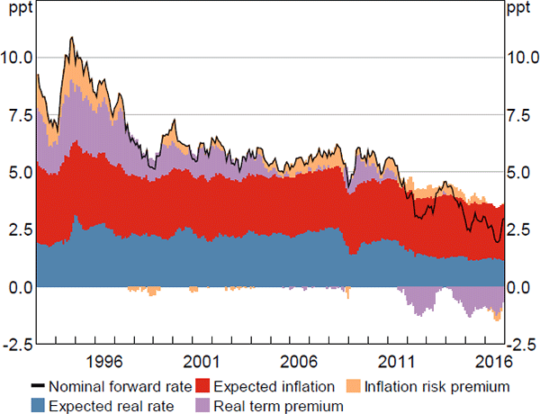
Figure 3 shows the decomposition of five-year-ahead nominal forward rates. Nominal forward rates have declined consistently over the sample period, largely reflecting declining real term premia and inflation risk premia. In comparison, expected real and inflation rates have been more stable, although have nonetheless also declined somewhat relative to the levels in the 1990s. We discuss each of these in more detail below.
Focusing first on expected short-term nominal interest rates, estimated expectations have declined since the early 1990s (Figure 4). The initial decline coincided with a shift lower in inflation, associated with the introduction of inflation targeting by the Reserve Bank, while rates declined further in the period following the global financial crisis. More broadly, expected nominal interest rates follow a generally procyclical pattern and ten-year-ahead expected rates tend to be less volatile than shorter tenor expectations, as anticipated.
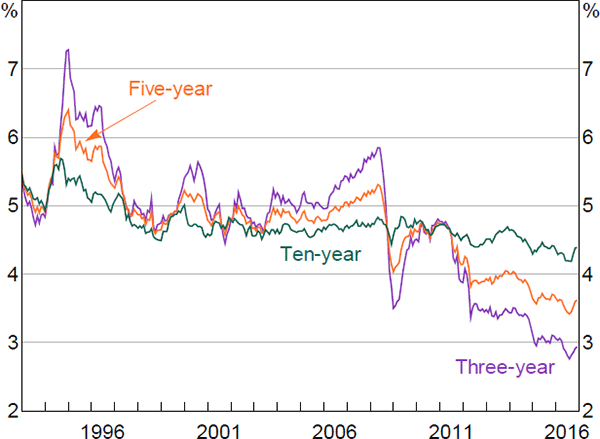
The estimates follow a very similar pattern to Jennison (2017), and also to that implied by a purely nominal model that we estimated using a similar methodology.[20] This provides a good crosscheck. It also suggests that we don't lose much information when using a simpler nominal model and so it may be preferable to use such a model when we are only interested in developments in nominal rates.
Expected inflation was relatively high and volatile early in the sample, but has fallen and become more stable over time (Figure 5). In particular, inflation expectations decreased substantially after the introduction of the inflation-targeting regime in the mid 1990s, though, consistent with other analyses (e.g. Finlay and Wende 2012; Moore 2016), the results suggest that it took a number of years for expectations to become anchored around the target. The fact that inflation expectations jump prior to the introduction of the goods and services tax (GST) in July 2000 appears to, in part, reflect data issues. Specifically, there were no inflation-indexed bonds with relatively short maturities trading at this time. As such, the real yield data would not be providing any useful information to help the model evaluate the temporary nature of any increase in inflation expectations.[21] The spike in ten-year-ahead inflation expectations in 2009 is somewhat surprising, although it is borne out in the survey data.[22] The model suggests that expectations of future inflation a number of years out have declined a bit over recent years, but that the decline is modest and that expectations have remained entrenched in the target range of 2 to 3 per cent.
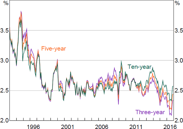
Interestingly, the estimates of expected inflation are more volatile than those from Finlay and Wende (2012), especially at long horizons. In part, this seems to reflect the fact that the model puts a greater weight on the five-year five-year forward survey data on inflation expectations, which were relatively volatile early in the sample. Nevertheless, the overall profile is similar between the two models.
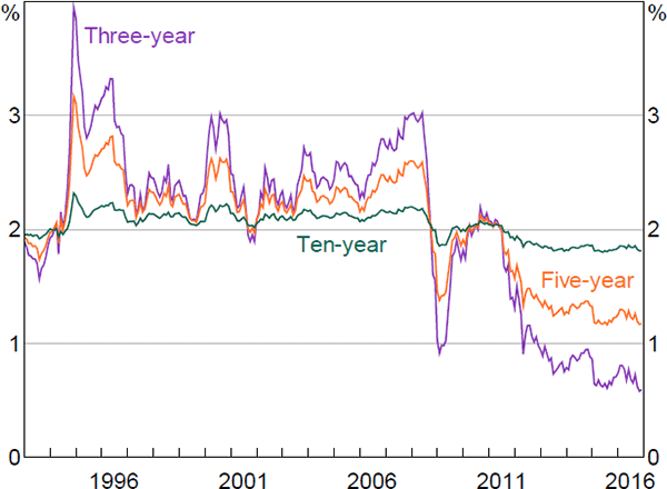
Estimates of expected future real short-term interest rates have also declined somewhat over recent years (Figure 6). For example, estimated five-year-ahead real rates have declined by around 1 percentage point since 2011, while ten-year-ahead real rates have declined by around ¼ percentage point. As these reflect expectations of real short-term interest rates in the relatively distant future, they can be interpreted as market measures of the neutral real interest rate (e.g. Christensen and Rudebusch 2017). As such, the results suggest that Australian neutral real interest rates have declined over recent years, though the decline implied by these market measures is muted relative to the decline implied by some other measures.[23]
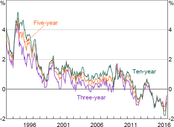
Shifting to term premia, the nominal term premia in Figure 7 (real plus inflation risk premium) declined in the early to mid 1990s, and remained low during the mid 2000s when uncertainty regarding inflation and growth, measured as the dispersion of analyst forecasts, was relatively low. This period is also referred to as the ‘Great Moderation’. The premia spike at the onset of the global financial crisis, a period of heightened economic uncertainty, and again in 2013 during the so-called ‘taper tantrum’ in the United States, when yields on US government bonds increased sharply in response to suggestions that the Federal Reserve would taper its quantitative easing program. Notwithstanding these episodes, premia have been particularly low for most of the period since the financial crisis. This could reflect spillovers from foreign central bank quantitative easing programs, which have been found to affect Australian bond markets through the so-called ‘portfolio balance’ channel (e.g. Bauer and Neely 2014; Neely 2015).
The influence of overseas developments is more evident in Figure 8, where we plot our estimates of 10-year average nominal term premia alongside two sets of estimates for the United States: one produced by the New York Federal Reserve, using the methodology laid out in Adrian et al (2013); and the other produced by the Board of Governors of the Federal Reserve System, using the methodology laid out in Kim and Wright (2005).[24] All three series follow broadly similar paths, though our estimates follow those from Kim and Wright particularly closely. The fact that our estimates of term premia for Australia are below those for the United States for at least part of the sample is somewhat surprising, though it is also the case for the estimates from Finlay and Chambers (2009) and Jennison (2017). One explanation could be the relative scarcity of AGS, particularly given there are relatively few other AAA-rated Australian dollar-denominated securities available. Another could be that the US models do not account for the zero lower bound, and this could be affecting estimated US term premia. In any case, one should not place too much weight on the precise estimated level of the series.
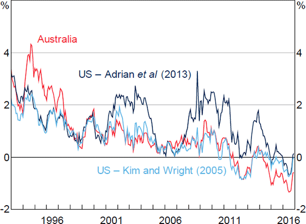
Sources: Authors' calculations; Board of Governors of the Federal Reserve System; Federal Reserve Bank of New York; Federal Reserve Bank of St. Louis
Our estimates of nominal term premia are broadly similar to those in Jennison (2017), although some differences exist: our measure spikes more sharply in 2009 during the peak of the financial crisis and in 2013 during the taper tantrum, and is slightly lower during the mid 2000s. It appears that these differences reflect the use of surveys to ameliorate the small-sample issues, rather than bootstrapping, and not the fact that we estimate a joint model of nominal and real yields instead of a purely nominal model.[25]
To get a better understanding of the evolution of nominal term premia, we can examine its components: the real term premium and the inflation risk premium. Real term premia declined during the late 1990s and early to mid 2000s (Figure 9), which coincided with a period of relatively strong economic growth and falling unemployment. The particularly sharp decline in real term premia in the early to mid 2000s has been documented for the United States (Abrahams et al 2016) and the United Kingdom (Joyce, Kaminska and Lildholdt 2012). Some have attributed it to a global ‘search for yield’ associated with perceptions of greater macroeconomic stability and excess liquidity (Joyce et al 2012). Real term premia also declined sharply over the early years of the financial crisis, and appear to have driven most of the decline in nominal term premia seen during this period. This is consistent with Abrahams et al (2016) finding that the Federal Reserve's quantitative easing program primarily lowered real term premia.
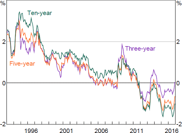
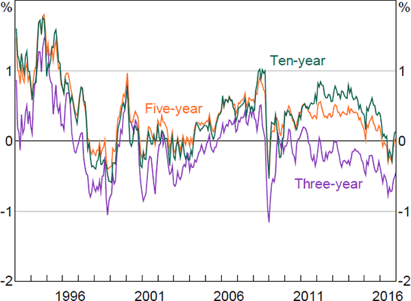
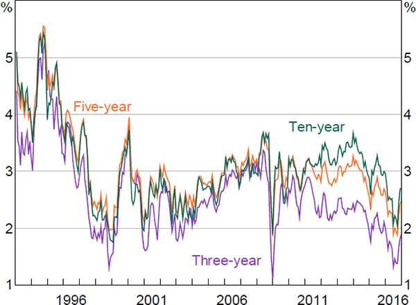
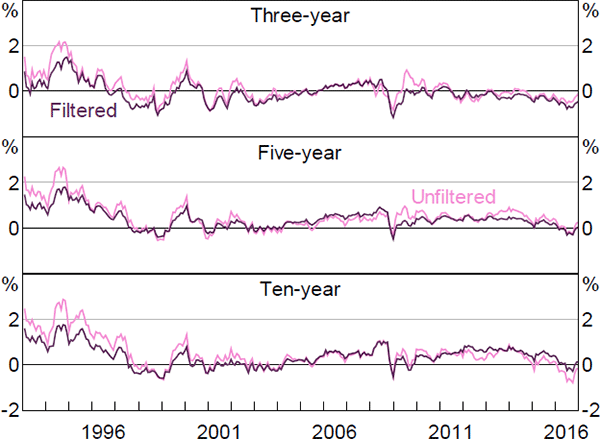
Estimated inflation risk premia (Figure 10) are reasonably similar to those estimated in Finlay and Wende (2012). Inflation risk premia declined sharply in the mid to late 1990s. This coincided with a sharp decline in survey measures of both uncertainty regarding future inflation and of expectations for the level of inflation as the Reserve Bank's inflation target gained credibility. Inflation risk premia spiked temporarily around the introduction of the GST. They were also quite volatile around the start of the global financial crisis, with three-year premia in particular first falling sharply and then rising. Christensen, Lopez and Rudebusch (2010) observe a similar phenomenon around the crisis with US data, and suggest that, similar to the discussion above, a sharp fall in the relative liquidity premium associated with nominal bonds over inflation-indexed bonds manifested in a lower inflation risk premium, which was subsequently unwound as liquidity returned to the inflation-indexed bond market. We can also see that much (although not all) of the decline and subsequent reversal in break-even inflation rates around 2016 seems to have reflected movements in inflation risk premia (Figures 10 and 11). This could reflect changes in uncertainty regarding future inflation outcomes, or potentially changes in the relative liquidity premium for inflation-indexed versus nominal bonds.
Overall, and similar to Abrahams et al (2016), our results suggest that while expectations for future short-term nominal, real and inflation rates vary over time, changes in risk premia tend to have a greater influence than changes in expectations on movements in observed yields and measures of break-even inflation, at least over short time horizons. This emphasises the importance of not taking changes in observed yields at face value when trying to infer market expectations.
5. Robustness Checks
5.1 Sample Starting in 1997
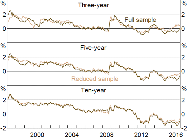
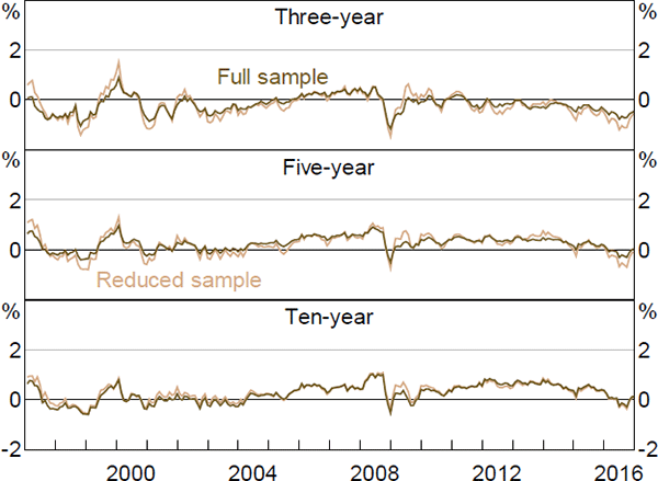
The data sample used in Section 4 spans the period before and after the Reserve Bank adopted a formal 2 to 3 per cent inflation target. Therefore, there could be a structural break, or regime shift, for which the model does not adequately account. This would be of particular concern given that the model imposes stationarity. To check the robustness of the results, we estimate the model on a reduced sample beginning in 1997, once inflation expectations had become reasonably anchored.[26]
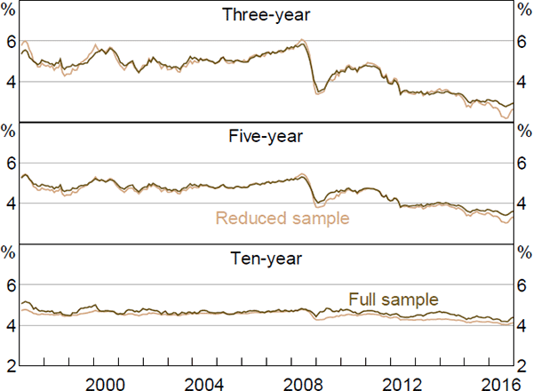
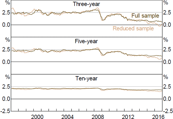
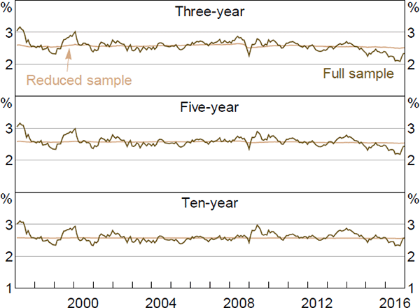
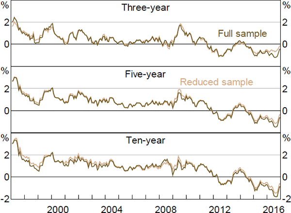
Nominal and real interest rates, and term premia, follow fairly similar paths to those estimated using the full sample, although expected rates tend to be smoother, especially at longer horizons (Figures E1–E6). In particular, ten-year-ahead nominal and real forward rates are a bit less variable when estimated over the shorter sample, while three- and five-year-ahead real rates show larger declines in recent years. The same is broadly true of inflation expectations, although the smoothness occurs to an even larger degree. Given the results for nominal and real expectations, this last point is perhaps not surprising: expected inflation is calculated as the difference between nominal and real expectations; if these expectations follow similar trends and are relatively smooth, then their difference will tend to be even smoother and flatter still.
More broadly, the smoothness is suggestive of a short-sample problem leading to insufficiently persistent pricing factors. In particular, Guimarães (2016) argues that discarding part of the sample due to changes in the structure of the economy is exactly the opposite of what we should do, as this variation can be extremely useful in separately identifying the P and Q dynamics. This argument could certainly be put forward here. By removing the early period we are potentially removing a period with a large amount of information about the dynamics of inflation expectations, and in particular how they become anchored (and therefore can potentially become unanchored). Nonetheless, both sets of results show broadly similar trends over time for a number of variables, which is reassuring.
5.2 Filtered versus Unfiltered Results
As noted in Section 3.1, we estimate the model in two steps: first we maximise the model's likelihood conditional on the observed factors; second we cast the model in a Kalman filter and re-optimise. The second step allows us to relax the assumption that the factors are priced correctly, and to drop any estimated zero-coupon real yield data that does not have a traded bond with a similar maturity and so is dependent on interpolation. Both of these generalisations are potentially important given the sparsity of inflation-linked bonds. Related to this, by using the Kalman filter and allowing for imperfect pricing in the factors, we allow the surveys to influence these pricing factors, which is also potentially important.
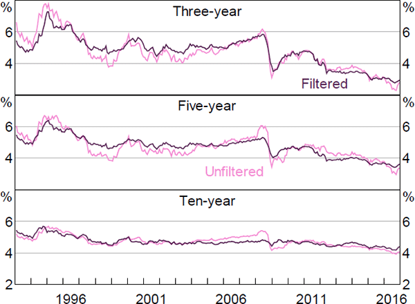
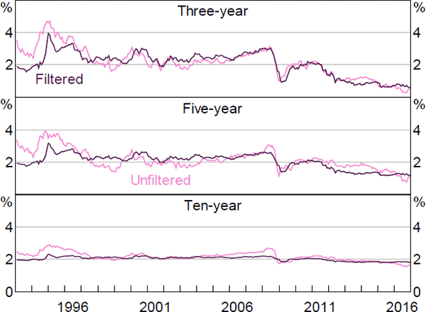
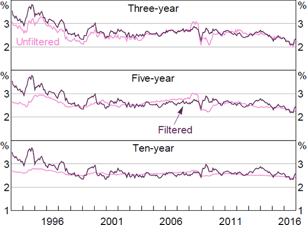
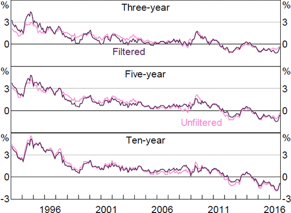
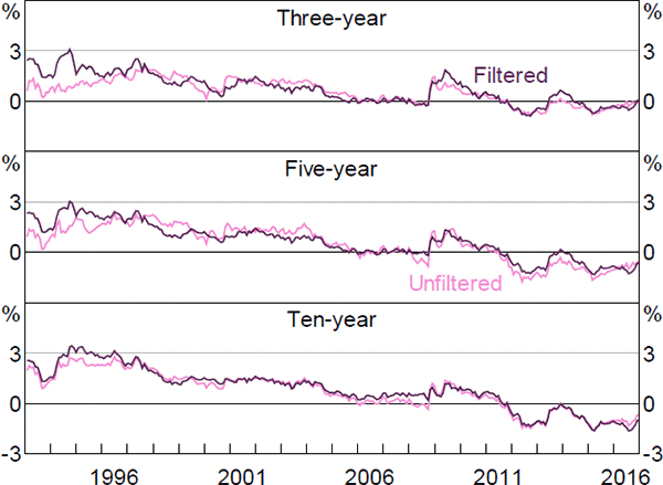
It is interesting to consider what the results would look like if we did not incorporate the second step. Figures F1–F6 contain these results. Again, the estimates of real and nominal interest rates and risk premia are broadly similar, while the estimates of expected inflation show greater differences. In particular, the inflation estimates are generally somewhat smoother, particularly the ten-year-ahead expectations, and there is a larger fall around the onset of the global financial crisis, although the broad trends are still reasonably similar and the results still suggest that inflation expectations are well anchored within the 2 to 3 per cent target band.
The inflation expectation estimates from the first step are also more similar to those from Finlay and Wende (2012). As with the estimates from that paper, the difference seems to be that the Kalman filtered model puts a higher weight on the surveys, as it estimates the variance of the noise associated with the surveys to be lower.[27] This appears to reflect the fact that the Kalman filter approach allows the surveys to affect the estimated pricing factors, rather than constraining the model to use the observed factors. The results are similar whether or not we drop some real yield data, suggesting that fully utilising the information contained in the survey data is the more important generalisation.
The fact that the filtered model places a greater weight on the surveys is particularly evident in Figure F7, which plots the model-implied inflation expectations for both the filtered and unfiltered models alongside the (closest) matching surveys. This also highlights the fact that even in the filtered model, the model-implied expectations do not perfectly coincide with the surveys and that they are taking a substantial signal from the yield data.
Overall, these results suggest that using a Kalman filter, and therefore allowing for pricing factors that diverge from the principal components of the yield data, can lead to a higher weight being put on surveys (though this will not necessarily be a general result). To the extent that we think surveys are good measures of market participants' expectations, this will be preferable. This will be particularly true if we are concerned about the quality of the real yield data, as may be the case in countries with a scarcity of inflation-indexed bonds. However, if for some reason we think that the surveys are a poor measure of expectations, for the full sample or even for some sub-sample, it may be preferable to eschew the Kalman filter or to calibrate the model to place a lower weight on the surveys.
6. Conclusion
The model described in this paper can provide policymakers with market-implied measures of expectations for a number of key economic variables. The model provides plausible estimates, though it should be noted that the estimates are subject to a degree of uncertainty and so one should focus on the broad trends implied by the model rather than any specific point estimate.
The model suggests that expected real rates a number of years in the future, a market-based measure of the neutral real interest rate, have declined since the global financial crisis. Meanwhile, longer-term inflation expectations have remained within the 2 to 3 per cent target band and have been more stable than suggested by other measures such as break-even inflation.
The results also show that nominal term premia declined over the sample and that this occurred in two distinct phases. The decline over the mid-to-late 1990s and early 2000s reflected declines in both real and inflation risk premia, and coincided with the implementation of the Reserve Bank's inflation-targeting regime as well as reasonably strong and stable economic performance. The decline since the crisis mainly reflects lower real term premia and may reflect overseas factors given it has coincided with declines in US term premia.
Appendix A: The Affine Term Structure Model
This section documents the mathematics of the ATSM that we use, and follows the expository style and terminology of Ang and Piazzesi (2003) closely.
First we derive pricing equations for the general class of ATSM that we use. Let  be the price of a nominal bond at time t that pays one dollar at time t + n. The no-arbitrage assumption implies that an equivalent martingale (or risk-neutral) measure, denoted by Q, exists such that
where rt is the nominal short rate (Harrison and Kreps 1979). Assume that the nominal short rate is given by  , where Xt is a stochastic process that describes all economic and financial factors relevant to bond pricing and which evolves according to
for μ a vector, θ and ∑ matrices, and εt+1 ~N(0,IN). Now denote the Raydon-Nikodym derivative, which converts the risk-neutral measure to the real-world measure, by ξt + 1; for any random variable Zt + 1,
where  without a superscript is understood to be under the real-world measure. In our case, we assume that the so-called market price of risk is given by
for λ0 a vector and λ1 a matrix, and that the Raydon-Nikodym derivative linking the real-world and risk-neutral measures is given by
Note that  is often referred to as the pricing kernel or stochastic discount factor, which summarises how agents discount pay-offs under different states of the world.
Given the above, we now show by induction that bond prices are exponentially affine in Xt. Assume that  ; we will show that this implies that
  . Starting from Equation (A1),
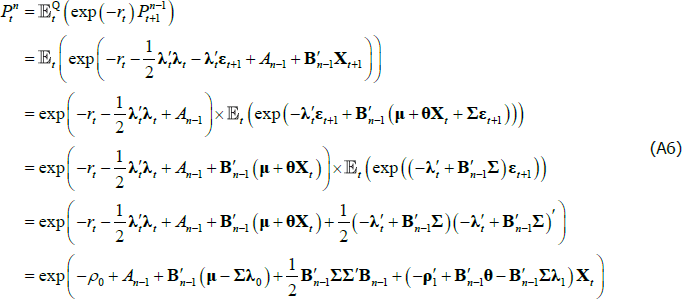
where line 2 follows from Equations (A3) and (A5) and the assumption that  , line 3 follows from Equation (A2), line 5 follows from the moment-generating function of a multivariate N(0,IN) random variable, and line 6 follows from Equation (A4) and the assumed functional form of rt. Line 6 has the desired functional form of exp
 , and so by equating coefficients that do and do not depend on Xt we can deduce that
To start the induction and also provide starting values for the above recursion, note that  , which implies that A0 = 0, B0 = 0. One can also directly calculate
  so that A1 = −ρ0 and B1 = −ρ1.
Next consider an inflation-indexed bond  that pays one unit of consumption good, or Qt + n/Qt units of nominal value, at time t + n. Here Qt is the price level, we define inflation πt by Qt/Qt – 1 = exp(πt), and we assume that
for π0 a scalar and π1 a vector. As with the nominal case, start by assuming that  . We will show by induction that this implies that
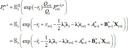
  . The no-arbitrage condition for an inflation-indexed bond is given by
where, using the fact that  , we define
  and
and  . But, given these re-definitions, the last line now matches line 2 from the nominal bond case, so that
To provide starting values for the above recursion, note that  , which implies that
  .
.
Two things are worth noting. First, in the pricing equations above, the price of risk parameters λ0 and λ1 are confounded with the factors describing the evolution of Xt, being μ, θ and ∑. As such, a cross-section of bond prices is not enough to fully identify the model. Second, and related to the first point, one would obtain the same pricing equations if one assumed that investors were risk neutral (so that λ0 = 0, λ1 = 0) and  for
for  and
and  .
.
Appendix B: The JSZ Normalisation
To estimate the model we need to impose some parameter restrictions to ensure econometric identification. There are a number of different normalisations one can use; we use that from JSZ for the reasons outlined in the main text. The JSZ normalisation is formulated for standard nominal ATSMs rather than joint nominal–real models, and is not set up to incorporate survey data. As such, we need to adapt JSZ to deal with real yields and survey data, which we do now.
Focusing first on the result from JSZ regarding estimation with observable factors in which separation of P and Q parameters in estimation is achieved (‘Case P’ in JSZ), Proposition 1 of JSZ gives the key result that any standard ATSM with the representation
is equivalent to a re-parameterised model with the representation
where  is a scalar, J(λQ) is a diagonal matrix,
  is a lower triangular matrix and 1′ is a vector of ones. The nominal part of our model fits within this framework. To incorporate the real part of our model we need to know how the inflation equation (Equation (A7)) maps between the standard and JSZ representations. But Equation (A17) of JSZ shows how to map from JSZ parameters
  to standard parameters (ρ0, ρ1):
where C and D are functions of the model parameters (see also Equations (15) and (16) in Proposition 2 of JSZ). The inflation equation  has the same functional form as
  , and so the mapping is given by Equation (B1) also. Reversing the mapping, if one starts with
  in the JSZ representation, that is
  , this maps back to (π0, π1) in the standard representation so that
  as desired.
The survey data are assumed to be noisy observations on the true underlying expectations for short-term interest rates or the inflation rate. Focusing on the inflation rate (the short-term interest rate case is the same), we have that  so that
  .
.
But iterating forward Equation (A2),  and so we can express the survey data in terms of underlying model parameters (representing true expectations) and some (assumed) normally distributed error term. We include the likelihood of the survey data along with those of the pricing factors and the bond yields in the numerical optimisation. For the case of estimation with observable factors, the survey data is allowed to affect estimates of the parameters but not the factors themselves, as these are constrained to be the principal components of the bond yields (for a yield-only model this is actually no constraint at all, but for a model with surveys it does impose constraints). But in fact, since expectations of short-term interest rates and the inflation rate depend on the future expected value of the pricing factors, the survey data also contains information on these pricing factors. We allow for this in the Kalman filter framework where factors are not directly observable and must be estimated (‘Case F’ in JSZ). This means that we no longer achieve separation of P and Q parameters in estimation, but the dependence is nonetheless relatively weak which, combined with good starting values from the estimation using observable factors, results in a relatively easy-to-estimate model.
Appendix C: Estimating the Real Zero-coupon Yield Curve
Unlike nominal bonds, there are relatively few inflation-indexed bonds on issue for the majority of our sample period, which makes estimating a zero-coupon real yield curve difficult. In particular, between 1992 and 2011 there are between two and three inflation-indexed bonds with residual maturity between 1 and 15 years outstanding at any one time, while from 2012 there are four to five such bonds outstanding at any one time. This low number makes fitting a flexible yield curve problematic, as arbitrary choices in yield curve modelling can have a non-negligible impact on the estimated curve shape.
To alleviate this problem we choose a particularly simple and transparent yield curve fitting method: interpolating the forward rate between outstanding bonds. So, for example, if the shortest-to-maturity inflation-indexed bond has two years until maturity and a yield of 1 per cent, we set the forward rate out to two years at 1 per cent. We then calculate what forward rate is required to price the next bond on the yield curve correctly, taking into account the previously estimated forward rates, continuing until all bonds are priced. This delivers estimated zero-coupon forward and yield curves that minimise spurious ‘wiggles’ and that price all outstanding bonds correctly.
For the ATSM we only use yield data for tenors where we have an outstanding bond, and do not use yield data interpolated between bond maturities, which further minimises the effect of the zero-coupon yield curve estimation on our final results.
In addition, we adjust the estimated zero-coupon real yield curve for the effects of known, lagged inflation on bond prices. The observed price, and so yield, of inflation-indexed bonds depends on past inflation a little. In particular, the cash flows of an inflation-indexed bond are determined by realised inflation ending two quarters before the quarter of the cash flow (so if the bond pays a coupon in November – that is, the December quarter – then the payout is based on inflation up until the end of the June quarter). Similarly, the bond price formula linking quoted real yields to bond prices in dollar terms depends on a cumulative inflation factor that is updated daily but is predictable up to a quarter and a bit in advance, with the degree of predictability determined by where in the quarter one is. This predictability will be incorporated into market prices and so will distort observed real yields: for example, a high inflation read will boost the nominal value of a real bond (since the bond's payouts will be boosted by the high inflation read once the pricing formula fully updates), and so will tend to push down the observed real yield relative to a ‘true’ real yield based on only forward-looking expectations. We correct for this by pushing the real yield back up a bit.
Consider an inflation-indexed bond paying real coupons Si at time i (where the final face value payment is included in the Si), let P be the price of this bond today, let πa,b be the cumulative inflation between a and b, where time is measured relative to today, let yi be the nominal yield, and let  be the unobserved ‘true’ real yield that would be observed if inflation-indexed bonds did not suffer from indexation lag. We will recover
  by writing the observed bond price P as a function of known inflation and nominal yields, and the unknown true real yield, and solving for the latter. In particular, by summing up nominal cash flows we can write
where the first two terms in the sum on the right give the nominal value of the real coupons after adjusting for cumulated inflation, and the third term is the nominal discount factor, where Δ is the indexation lag. Now for i ≤ Δ, π− Δ,i − Δ is known and we write  to distinguish this. For i > Δ,
where the last line follows from expressing the real yield in terms of the expected value of cumulated inflation discounted by a nominal yield. As such, letting  represent coupons that are currently known and
  represent coupons that depend on future inflation, we can write the inflation-indexed bond price P as
where  for those coupons where inflation is known, and we define
  for those coupons that depend on future unknown inflation (as well as some lagged inflation). As the yi can be estimated from nominal yield curve data,
  is the only unknown quantity above and we can solve for it numerically; differences between the observed real yield and the ‘true’ real yield that we estimate will be driven by (i) observed inflation via π−Δ,0, and (ii) the level and slope of the nominal yield curve via yi.
In practice, the inflation-indexed bond pricing formula linking quoted real yields to actual bond prices is updated with half the increase in the past two quarters' CPI reads, so as well as knowing one or two pricing formula updates perfectly in advance, we also know an additional ‘half’ of a pricing formula update. We treat the case as we do for the known formula updates ( above), but in this case the π−Δ,i − Δ factor is half known and half solved for in estimation, with the unknown inflation component taken as the relevant nominal yield less the fitted real yield, using the identity that nominal = real + inflation.
Appendix D: Descriptive Statistics
| 6 | 12 | 18 | 24 | 36 | 48 | 60 | 84 | 120 | 180 | |
|---|---|---|---|---|---|---|---|---|---|---|
| Nominal | ||||||||||
| Mean (ppt) | 4.75 | 4.80 | 4.85 | 4.91 | 5.06 | 5.20 | 5.32 | 5.49 | 5.66 | na |
| Standard deviation (ppt) | 1.62 | 1.69 | 1.74 | 1.77 | 1.81 | 1.83 | 1.84 | 1.84 | 1.81 | na |
| Autocorrelation | 0.988 | 0.985 | 0.984 | 0.984 | 0.986 | 0.987 | 0.988 | 0.988 | 0.988 | na |
| Real | ||||||||||
| Mean (ppt) | na | na | na | 2.63 | 2.67 | 2.71 | 2.75 | 2.81 | 2.86 | 2.91 |
| Standard deviation (ppt) | na | na | na | 1.35 | 1.37 | 1.39 | 1.39 | 1.32 | 1.36 | 1.27 |
| Autocorrelation | na | na | na | 0.990 | 0.991 | 0.992 | 0.992 | 0.992 | 0.991 | 0.990 |
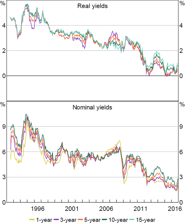
Sources: Authors' calculations; RBA
Appendix E: Estimated Forward Rates for Reduced Sample
Appendix F: Estimated Forward Rates for the Unfiltered Model
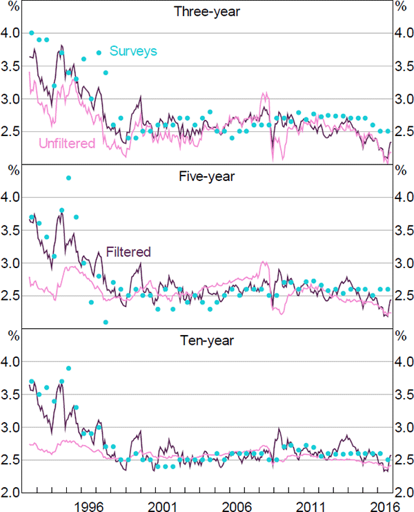
Note: Ten-year-ahead survey observations are taken as five-year five-year forward expectations
Sources: Authors' calculations; Consensus Economics
References
Abrahams M, T Adrian, RK Crump, E Moench and R Yu (2016), ‘Decomposing Real and Nominal Yield Curves’, Journal of Monetary Economics, 84, pp 182–200.
Adrian T, RK Crump and E Moench (2013), ‘Pricing the Term Structure with Linear Regressions’, Journal of Financial Economics, 110(1), pp 110–138.
Ang A and M Piazzesi (2003), ‘A No-Arbitrage Vector Autoregression of Term Structure Dynamics with Macroeconomic and Latent Variables’, Journal of Monetary Economics, 50(4), pp 745–787.
Bauer MD and JD Hamilton (2017), ‘Robust Bond Risk Premia’, Federal Reserve Bank of San Francisco Working Paper 2015-15, rev.
Bauer MD and CJ Neely (2014), ‘International Channels of the Fed's Unconventional Monetary Policy’, Journal of International Money and Finance, 44, pp 24–46.
Bauer MD, GD Rudebusch and JC Wu (2012), ‘Correcting Estimation Bias in Dynamic Term Structure Models’, Journal of Business & Economic Statistics, 30(3), pp 454–467.
Bibkov R and M Chernov (2011), ‘Yield Curve and Volatility: Lessons from Eurodollar Futures and Options’, Journal of Financial Econometrics, 9(1), pp 66–105.
Buraschi A and A Jiltsov (2005), ‘Inflation Risk Premia and the Expectations Hypothesis’, Journal of Financial Economics, 75(2), pp 429–490.
Chernov M and P Mueller (2012), ‘The Term Structure of Inflation Expectations’, Journal of Financial Economics, 106(2), pp 367–369.
Christensen JHE, JA Lopez and GD Rudebusch (2010), ‘Inflation Expectations and Risk Premiums in an Arbitrage-Free Model of Nominal and Real Bond Yields’, Journal of Money, Credit and Banking, 42(Supplement s1), pp 143–178.
Christensen JHE and GD Rudebusch (2017), ‘A New Normal for Interest Rates? Evidence from Inflation-Indexed Debt’, Federal Reserve Bank of San Francisco Working Paper 2017-07.
Cochrane JH (2001), Asset Pricing, Princeton University Press, Princeton.
Cochrane JH and M Piazzesi (2005), ‘Bond Risk Premia’, The American Economic Review, 95(1), pp 138–160.
Dai Q and KJ Singleton (2000), ‘Specification Analysis of Affine Term Structure Models’, The Journal of Finance, 55(5), pp 1943–1978.
Duffee GR (2002), ‘Term Premia and Interest Rate Forecasts in Affine Models’, The Journal of Finance, 57(1), pp 405–443.
Duffie D and R Kan (1996), ‘A Yield-Factor Model of Interest Rates’, Mathematical Finance, 6(4), pp 379–406.
Finlay R and M Chambers (2009), ‘A Term Structure Decomposition of the Australian Yield Curve’, Economic Record, 85(271), pp 383–400.
Finlay R and S Wende (2012), ‘Estimating Inflation Expectations with a Limited Number of Inflation-Indexed Bonds’, International Journal of Central Banking, 8(2), pp 111–142.
Guimarães R (2016), ‘Fool's Errand? Robust Identification of Risk Premia and Expectations in Asset Prices’, Unpublished manuscript, Bank of England, May. Previously released as Bank of England Working Paper No 489.
Hamilton JD and JC Wu (2012), ‘Identification and Estimation of Gaussian Affine Term Structure Models’, Journal of Econometrics, 168(2), pp 315–331.
Harrison JM and DM Kreps (1979), ‘Martingales and Arbitrage in Multiperiod Securities Markets’, Journal of Economic Theory, 20(3), pp 381–408.
Jennison F (2017), ‘Estimation of the Term Premium within Australian Treasury Bonds’, Australian Office of Financial Management Working Paper 2017-01.
Joslin S, M Priebsch and KJ Singleton (2014), ‘Risk Premiums in Dynamic Term Structure Models with Unspanned Macro Risks’, The Journal of Finance, 69(3), pp 1197–1233.
Joslin S, KJ Singleton and H Zhu (2011), ‘A New Perspective on Gaussian Dynamic Term Structure Models’, The Review of Financial Studies, 24(3), pp 926–970.
Joyce MAS, I Kaminska and P Lildholdt (2012), ‘Understanding the Real Rate Conundrum: An Application of No-Arbitrage Models to the UK Real Yield Curve’, Review of Finance, 16(3), pp 837–866.
Kim DH and A Orphanides (2012), ‘Term Structure Estimation with Survey Data on Interest Rate Forecasts’, Journal of Financial and Quantitative Analysis, 47(1), pp 241–272.
Kim DH and JH Wright (2005), ‘An Arbitrage-Free Three-Factor Term Structure Model and the Recent Behavior of Long-Term Yields and Distant-Horizon Forward Rates’, Board of Governors of the Federal Reserve System Finance and Economics Discussion Series No 2005-33.
Krippner L (2013), ‘A Tractable Framework for Zero Lower Bound Gaussian Term Structure Models’, Reserve Bank of New Zealand Discussion Paper DP2013/02.
Krippner L (2015), Zero Lower Bound Term Structure Modeling: A Practitioner's Guide, Applied Quantitative Finance, Palgrave Macmillan, New York.
Li C, A Meldrum and M Rodriguez (2017), ‘Robustness of Long-Maturity Term Premium Estimates’, Board of Governors of the Federal Reserve System, FEDS Notes, 3 April.
Malik S and A Meldrum (2016), ‘Evaluating the Robustness of UK Term Structure Decompositions Using Linear Regression Methods’, Journal of Banking & Finance, 67, pp 85–102.
McCririck R and D Rees (2017), ‘The Neutral Interest Rate’, RBA Bulletin, September, pp 9–18.
Moore A (2016), ‘Measures of Inflation Expectations in Australia’, RBA Bulletin, December, pp 23–31.
Neely CJ (2015), ‘Unconventional Monetary Policy had Large International Effects’, Journal of Banking & Finance, 52, pp 101–111.
Vlieghe G (2017), ‘Real Interest Rates and Risk’, Speech given at The Society of Business Economists Annual Conference ‘Challenge and Change – The UK, Euro Area and Global Economic Outlook’, London, 15 September.
Footnotes
For a further discussion in the Australian context, see McCririck and Rees (2017). See also Vlieghe (2017) for an excellent discussion of the determinants of real interest rates from a macrofinance perspective. [1]
Guimarães (2016) also estimates a joint model using an extension of the JSZ approach, although fewer details are given and this is not the main focus of the paper. [2]
The relatively restrictive error assumption used here, and throughout the paper, is unlikely to hold in the data. While we could allow for more complex error structures, doing so would significantly increase the complexity of the model. Moreover, Bibkov and Chernov (2011) find that doing so helps models match higher-order moments of the data, but not the first moments (i.e. yields). [3]
An example of government bonds providing a form of insurance is the global financial crisis, which saw bond yields fall (and therefore bond prices rise) amid deteriorating economic circumstances. An example of the opposite is the 1970s, when relatively poor economic outcomes were accompanied by rising yields. [4]
Expected inflation and interest rates at long horizons are driven by the expected value, under the P dynamics, of the pricing factors. If the pricing factors mean-revert quickly under P dynamics, these values will simply converge to a constant. [5]
One potential concern with this approach is that the expectations of bond traders could differ from the expectations of survey participants. However, the literature tends to find that the two sets of expectations are consistent with each other (e.g. Chernov and Mueller 2012). [6]
We experimented with bootstrapping, but the estimated forward rates a number of years ahead appeared unreasonably volatile. [7]
For more details, see Appendix B. [8]
Consistent with papers such as Adrian et al (2013), Abrahams et al (2016) and Malik and Meldrum (2016), we constrain the steady-state level of the pricing factors to be their sample averages. This helps to avoid small-sample biases. [9]
We initialise the Kalman filter factors using the level of the observed principal component factors. We also use a few different starting points for the parameters based on the first step of the estimation to help ensure we find a global, not local, maximum. [10]
The results are, in fact, reasonably robust to not dropping these yields. [11]
While a number of papers have argued that yields are not ‘spanned’ by the first three principal components of the yield curve (e.g. Cochrane and Piazzesi 2005; Joslin, Priebsch and Singleton 2014), Bauer and Hamilton (2017) show that standard tests lack power, and that properly accounting for this leads to less evidence that three factors are insufficient. [12]
One could also extract pricing factors from a joint panel of nominal and real yield data, although in practice both methods deliver factors that are essentially linear combinations of the other, and both sets of factors explain over 99.9 per cent of the variation in the nominal and real yield data. [13]
Malik and Meldrum (2016) find that models that instead impose a unit root tend to perform poorly. [14]
See Appendix C for further details. Another approach would have been to use the indexed bond prices directly as in Finlay and Wende (2012). However, this approach is not well suited to the JSZ normalisation. It would also require a nonlinear Kalman filter. Given that we want the model to be simple enough to be used on an ongoing basis, we eschewed this option. [15]
Liaison suggests that inflation-linked bonds provide the most reliable information on expectations between around three and ten years. Nevertheless, we use a wider range of yields because of the sparsity of traded bonds. [16]
Although the pricing factors used in the final model are generated by the Kalman filter, and therefore, in principal, can differ substantially from the original factors (including in that we no longer enforce orthogonality), in practice they are very similar to the original factors and so for ease of exposition we refer to them interchangeably. [17]
Using the logic that ‘nominal = real + inflation’, one might expect the parameters associated with the nominal factors in π1 to be positive and the parameters associated with the factors extracted from real data to be negative, similar to how one calculates break-even inflation. This is not the case, as: (i) the situation is not quite as simple as the above equation implies as we are interested in specifying the short-term inflation rate, but we are using long-term yield data that includes term and risk premia as well as expectations; (ii) the pricing factors themselves have both positive and negative loadings on the underlying yield data (see Figures 1 and 2); and (iii) the real data are first orthogonalised with respect to the nominal factors. [18]
Recall that θ is defined via ΔXt + 1 = μ + θXt + ∑εt + 1 rather than the more traditional Xt + 1 = μ + θXt + ∑εt + 1; in the latter case, the estimated values of θ would be one unit higher for all diagonal entries. [19]
Specifically, we estimated a model of nominal rates using the methodology outlined in Adrian et al (2013), but extended to include cash rate forecasts. [20]
Measures of unions' long-term inflation expectations did increase sharply around this time, so it is conceivable that the spike is not purely a statistical artefact. [21]
Specifically, surveys of five-year five-year forward inflation expectations increase relative to expectations three to four years ahead; this implies a relatively large change in quite long-term expectations. [22]
For further analysis, see McCririck and Rees (2017). [23]
The Kim and Wright (2005) methodology incorporates surveys, while the Adrian et al (2013) methodology only uses yield data. For a more detailed comparison of the models and their estimates, see Li, Meldrum and Rodriguez (2017). [24]
We estimated a purely nominal model incorporating surveys of cash rate expectations, and the estimated term premia were very similar to those produced by the joint model. [25]
Another approach would be to estimate a model with regime switching. However, the added complexity this would involve was not in keeping with our focus on estimating a usable ‘workhorse’ model. [26]
On the flip side, it estimates the variance of the noise associated with the real yields to be higher. The estimates of the variance of the noise associated with the nominal yields are similar in the filtered and unfiltered models. [27]


